pnorm(-2.61, 0, 1, lower.tail = TRUE)[1] 0.004527111Single proportion
In this document, we are going to walk through, step-by-step, the fundamentals of hypothesis testing.
Suppose the Howling Cow company claims that 50% of NC State students eat Howling Cow at dinner. We think that less than 50% of students eat Howling Cow at dinner.
To test this, you take a random sample of 100 students, and are interested in if they had Howling Cow ice creme with their dinner or now. We observed 37 students have ice creme, and 63 students not have ice creme.
We can use the above context to start setting the stage for our hypothesis test. Some questions we need to ask ourselves include:
– What is our variable of interest? What type of variable is it?
– What is our population of interest?
– What assumption are we making about the population?
– What is our research question?
We can define our random variable (X) as:
X = If an NC State student eats Howling Cow ice creme at dinner
This is a categorical variable, and can be mapped to 0, 1 values as such.
\[ X = \begin{cases} 1 & \text{if yes}\\ 0 & \text{if no} \end{cases} \]
When we think about the term population, we can think about every observational unit that could be studied, or that we are interested in. In this situation, we are measuring if NC State students eat ice creme at dinner. The population we are interested in studying is all NC State students.
The assumption that we make about the population can fall into one of a few different categories:
– Assume that “nothing is going on”
– Assume an exsisting claim to be true
A common way to explain the first case is through the example of studying a coin that is 2-sided, and fair. If we assume that the coin really is fair, then we could make the assumption that the population proportion of times the coin lands on heads is 0.50 (50%).
In our ice creme context, we have an exsisting claim by the company that “Howling Cow company claims that 50% of NC State students eat Howling Cow at dinner”. This is what we will assume about the population when conducting our hypothesis test.
This assumption is called the null hypothesis. Because we are working with a categorical variable, and are at the population level, the proper notation is as follows:
\[ H_o: \pi = 0.5 \]
We again turn to the context to figure out our research question. We can think about our research question as what we are interested in investigating. In the case we are investigating: “We think that less than 50% of students eat Howling Cow at dinner”.
The research question is going to come in one of three directions:
– less (<)
– greater (>)
– different (\(\neq\))
We use the appropriate sign when writing out our alternative hypothesis. This is critical when we calculate the p-value later on.
\[ H_a: \pi < 0.5 \] Note: The null and alternative hypothesis will always have the same population parameter and same value.
To investigate into what’s happening at the population, we collect data from said population. In the above context, we observed that 37 NC State students eat Howling Cow ice creme at dinner, and 63 don’t. We know this is a categorical variable (defined above), and can write out our sample statistic as so:
\[ \hat{p} = \frac{37}{100} \]
In order to use theory based procedures, we have certain assumptions we need to check. For one categorical variable, we need to check:
– Independence assumption
– Sample size assumption
This assumption will be in ever inference tool we use this semester. We can define independence as “one observational unit not having influence/effecting another”. Although we can not strictly test for this, we can think about how we collect our data in order to justify this assumption.
– Do we have a random sample?
– Is this sample < 10% of the total population?
A random sample is where each observational unit has an equal chance of being selected. This is often difficult in practice. One way we could achieve this for NC State students, is to get a list of all students on a registry, and use a random number generator to select 100. We need to sample < 10% of the total population, so we don’t over sample, and mis-estimate the sampling variability (standard error assocciated with the sampling distribution).
Next, we need to check if we have a sufficiently large sample size. Recall that our goal is to create a null distribution, and check to see if our statistic is likely or unlikely to be seen under the assumption of the null hypothesis. Because our goal is to create a null distribution, we are going to check our sample size condition under the assumption of the null hypothesis. For this condition to be met, we need to have:
– 10 successes (what we are taking the proportion of)
– 10 failures
The null hypothesis states that the true proportion of NC State students who eat ice creme at dinner is = 0.5. So, would we expect to see more than 10 success and 10 failures from a sample size of 100 (same as our origional sample size) given this assumption is true?
\[ 100 * .5 = 50 expected successes > 10 \\ 100 * .5 = 50 expected failures > 10 \]
This condition is met! The central limit theorem is going to kick in, and our sampling distribution is going to be normal!
A null distribution is a sampling distribution of our statistic under the assumption of the null hypothesis that the true proportion of NC State students who eat ice creme is .50.
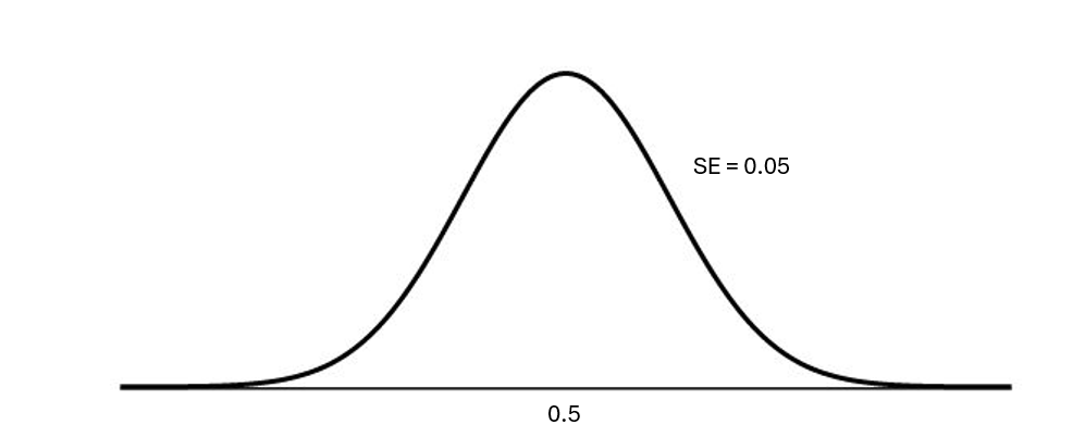
This sampling distribution is going to be centered at this value, because we make the assumption that the null hypothesis is true. What is the spread of this distribution going to be?
\[ SE = \sqrt{\frac{\pi_o * (1-\pi_o)}{n}} \]
Where
\[ \pi_o = the null value (0.50) \\ n = our sample size (100) \]
Plugging these values in, we get the following:
\[ SE = \sqrt{\frac{0.5 * (1-0.5)}{100}} = 0.05 \]
With this information, we can visualize the null distribution below:

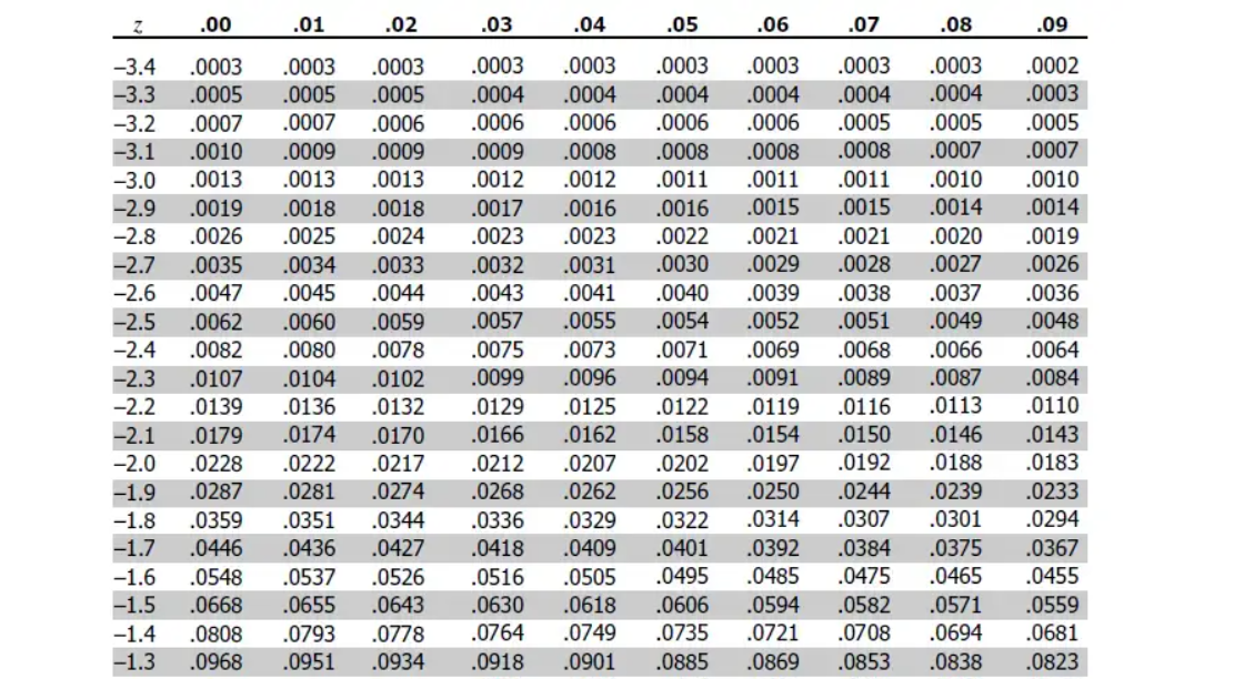
**Note: We could stop here and calculate our p-value. This is feasible because of technology. Hypothesis testing pre-dates computers, and when technology wasn’t as advanced, statisticians often would standardize their test statistic to follow a standard normal distribution, with pre-calculated probabilities.

Another benefit of standardizing your statistic is that:
– It gives us a nice interpretation
– It makes comparing across studies easier (because standardizing puts everything on the same scale)
We are going to calculate our standardized test statistic. We can standardize our test statistic to follow a standard normal distribution (Z-distribution). The standard normal distribution has a mean of 0, and a standard error of 1.
The reason why it’s a Z distribution (and not a t-distribution), is because we do not have to estimate the population standard deviation when working with categorical variables (and we do with quantitative variables). When working with categorical variables, each response is binned into a success or failure. We can have nothing in between. Thus, if we estimate the population proportion, we also know the population standard deviation. With quantitative variables, the population standard deviation is unknown, and must also be estimated. This extra layer of uncertainity is accounted for by using a t-distribution.
To standardize our statistic, we can do the following:
\[ Z = \frac{\hat{p} - \pi_o}{SE} \]
Plugging in these values, we get:
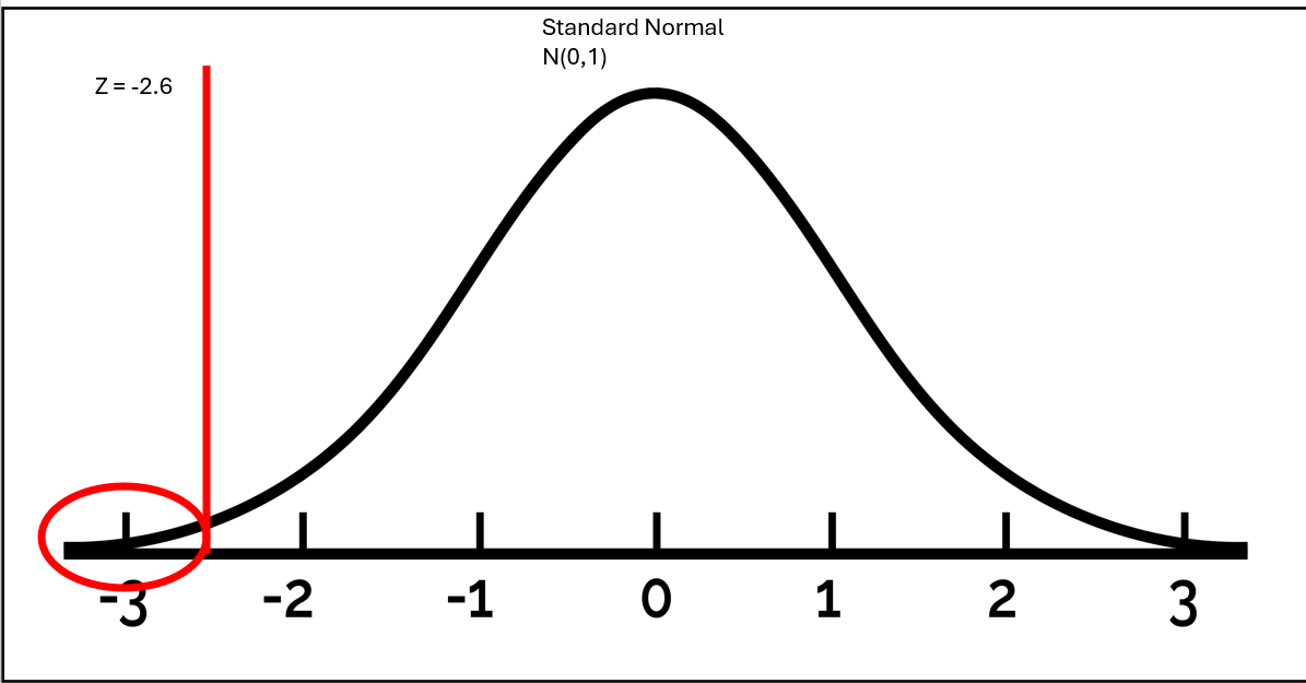
\[ Z = \frac{.37 - .5}{0.05} = -2.61 \]
We can visualize this as follows:

A p-value is the probability that we observe our statistic, or something more extreme, given that the null hypothesis is true. We can calculate a p-value using the pnorm function in R. The arguments are:
– statistic
– mean of distribution
– standard error
– lower.tail = [TRUE/FALSE]; where true looks left and false looks right
Using our standardize statistic, we find our p-value to be:
pnorm(-2.61, 0, 1, lower.tail = TRUE)[1] 0.004527111Note: This is the exact same value (besides rounding error on the standard error) if we used the distribution approximated in the Null Distribution section of this document:
pnorm(.37, .5, .05, lower.tail = TRUE)[1] 0.004661188In order to make a decision, we can compare our p-value to alpha. Alpha is a cut-off that suggests how much evidence we need to reject the null hypothesis. For this example, let’s assume that alpha = 0.05.
Because our p-value is smaller than alpha, we are able to reject the null hypothesis. This is our decision. If our p-value was larger than alpha, we would fail to reject the null hypothesis.
Our conclusion is always in terms of the alternative hypothesis. Because we have evidence to reject the null hypothesis, this also gives us strong evidence to conclude the altnerative hypothesis. Writing this in context, we can say that we have strong evidence to conclude that the true proportion of NC State students who eat ice creme at dinner is lower than 50%.
When you are asked to interpret the p-value, it’s asking you to explain the p-value using the exact definition. The definition of a p-value is the probability that we observe our statistic, or something more extreme, given the null hypothesis is true. Let’s add our context:
Interpretation: The probability of observing our sample statistic of .37, or something smaller, given that the true proportion of NC State students who eat ice creme is .50 is 0.004.
When we move to simulation studies:
– The assumptions are more relaxed
– We simulate the null distribution under the assumption of the null hypothesis to estimate the sampling distribution
– We do not standardize our statistic
Otherwise, we set up hypotheses the same, calculate p-values the same, and write evidence statements the same way!
We will spend a lot of time doing hypothesis testing in different situations (e.g. single mean, difference in proportions). The calculations and notation are going to slightly change, but the foundation of hypothesis testing (outlined above) remains the same.