library(palmerpenguins)
library(tidyverse)
library(tidymodels)
library(gridExtra)Theory based statistical inference
Difference in means
Packages
In this document, we are going to walk through, step-by-step, the fundamentals of hypothesis testing when working with a categorical explanatory variable, and a quantitative response variable.
Context
We are going to use a familiar data set (penguins) to demonstrate these theory based procedures. In this example, we are interested in exploring if the species of the penguin impacts the bill length (mm) of the penguin on the Palmer island. We will be looking at the Chinstrap and Gentoo species of penguin. We are interested in researching if there is a difference in bill length between the Gentoo penguins the Chinstrap penguins.
From this context, we can identify our two variables of species and bill length. Because of the language “species…impacts…bill length”, we can conclude that species is our explanatory variable. This can also be thought of as our grouping variable. bill length is the variable that we are interested in. It is a quantitative variable, meaning we are going to be working with means. Because we have a grouping variable (with two groups), we are going to be working with two means, and specifically looking at a difference in means.
Hypothesis Testing
In class, we set up the following null and alternative hypothesis
\[H_o: \mu_g - \mu_c = 0\]
\[H_a: \mu_g - \mu_c \neq 0\]
Recall that this is a test for independence. We assume (null hypothesis) that bill length is independent from species of penguin. We are researching if they are not independent, or that bill length really does depend on species. As a reminder for going forward, we can remind ourselves what the parameter of interest is:
\(\mu_g - \mu_c\) = the true mean bill length for the gentoo species minus the true mean bill length for the chinstrap species; the difference in true mean bill legnth between the gentoo and chinstrap species.
Because we are just looking for a difference, and don’t have a direction assocciated with our research question, our alternative hypothesis is two-sided (\(\neq\)).
Calculating the sample statistic
In class, we used the following code to calculate our sample statistic. Note that we now have two groups, which means we need to calculate two sample means!
penguins |>
  filter(species %in% c("Chinstrap", "Gentoo"),
         (!is.na(sex))) |>
  group_by(species) |>
  summarise(means = mean(bill_length_mm))
# A tibble: 2 × 2
species means
<fct> <dbl>
1 Chinstrap 48.8
2 Gentoo 47.6\(\bar{x}_g\) = 47.6
\(\bar{x}_c\) = 48.8
\(\bar{x}_g - \bar{x}_c\) = 47.6 - 48.8 = -1.2
Note That our order of subtraction is consistent with how we set up our null and alternative hypotheses! Order matters!
Assumptions
We again need to check assumptions to ensure that the central limit theorem kicks in, and that the sampling distribution of our difference in means under the assumption of the null hypothesis is ~ normally distributed.
Independence: As always, we need to check the independence assumption. For this situation, we need to check both within and across groups. That is, the penguins, within and between species, do not influence one another.
Normality: We check for skew and outliers for each group separately
When checking independence, the first thing we look for is any information on how the data were sampled. If the data come from a simple random sample, we have evidence to suggest that the independence assumption is not violated.
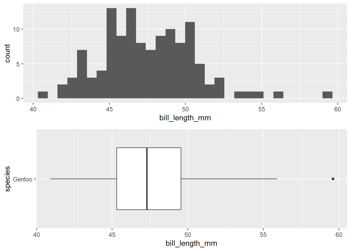
The following plots are for the gentoo species:
p1 <- penguins |>
  filter(species == "Gentoo") |>
  ggplot(
    aes(x = bill_length_mm)
  ) +
  geom_histogram()

p2 <- penguins |>
  filter(species == "Gentoo") |>
  ggplot(
    aes(x = bill_length_mm, y = species)
  ) +
  geom_boxplot()

grid.arrange(p1, p2, ncol = 1)
`stat_bin()` using `bins = 30`. Pick better value with `binwidth`.Warning: Removed 1 row containing non-finite outside the scale range
(`stat_bin()`).Warning: Removed 1 row containing non-finite outside the scale range
(`stat_boxplot()`).
# A tibble: 1 × 1
   size
  <int>
1   119
We can see from the above plot that there is some slight right skew in bill length for the gentoo species. However, with a sample size of 199, and only one outlier, this is not enough evidence to violate the normality assumption.
Let’s check the other species!
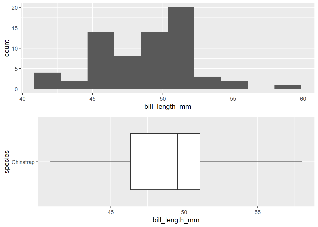
The following plots are for the chinstrap species:
p3 <- penguins |>
  filter(species == "Chinstrap") |>
  ggplot(
    aes(x = bill_length_mm)
  ) +
  geom_histogram(bins = 10)

p4 <- penguins |>
  filter(species == "Chinstrap") |>
  ggplot(
    aes(x = bill_length_mm, y = species)
  ) +
  geom_boxplot()

grid.arrange(p3, p4, ncol = 1)
# A tibble: 1 × 1
   size
  <int>
1    68
We seem some small evidence of left skew for bill length with the chinstrap species. However, there are no outliers, and our sample size is larger than 60. There is not enough evidence to suggest that normality is violated in this case.
Assuming independence, and having no evidence to suggest normality is violated, we know that our sampling distribution is going to be normal, and we can approximate the standard error of the sampling distribution using the following formula in the next section.
Estimating the Standard Error
The formula for a standard error in the difference in mean scenario is as follows:
\(\sqrt{\frac{s_1^2}{n_1} + \frac{s_2^2}{n_2}}\) where group 1 is our first group gentoo, and group 2 is our second group chinstrap.
We can calculate s (our sample standard deviations) and n (sample size) for each group using the code below:
penguins |>
  filter(species %in% c("Chinstrap", "Gentoo"),
         (!is.na(sex))) |>
  group_by(species) |>
  summarise(size = n(),
            spread = sd(bill_length_mm))
# A tibble: 2 × 3
species size spread
<fct> <int> <dbl>
1 Chinstrap 68 3.34
2 Gentoo 119 3.11We then take this information, and plug it into our equation above:
\(\sqrt{\frac{3.11^2}{119} + \frac{3.34^2}{68}}\) = 0.495
t-test
When working with a quantitative response, it is much easier to calculate a probability of interest when we standardize (versus working with proportions, where we showed two ways).
To calculate our t-statistic, we can use the following formula:
\(t = \frac{\bar{x}_g - \bar{x}_c - 0}{\sqrt{\frac{s_1^2}{n_1} + \frac{s_2^2}{n_2}}}\)
This follows the standard formula for a standardized statistic of:
\(\frac{stat - null}{SE}\).
We have calculated all of these values, and can plug them in to get our test statistic:
\(t = \frac{-1.2 - 0}{.495}\) = -2.42
This statistic suggests that our sample mean of -1.2 is 2.42 standard errors below the null value of 0.
Each t-distribution is different, and we need to specify our degress of freedom. The official formula for the degrees of freedom is quite complex so instead you may use the smaller of n1-1 and n2-1 for the degrees of freedom.
Recall that this is a two-sided test because of the alternative hypothesis, we we need to calculate the p-value looking at both sides of the distribution.
pt(-2.424, df = 67, lower.tail = T) * 2 #multiply by 2 because a t-distribution is symmetric[1] 0.01805622The book demonstrates the p-value calculation as follows. You may do either.
By setting the df = 67, it controls the shape (spread) of the distribution.
Decisions, conclusions, and interpretations.
Let’s assume that we are working with a \(\alpha = 0.05\) significance level. With a p-value of 0.018, we can say that:
Decision: Reject the null hypothesis
Conclusion: Strong evidence to conclude the alternative hypothesis that the true mean difference in bill length between gentoo and chinstrap is different than 0.
Interpretation: The probability of observing our sample mean difference in bill length of -1.2mm, or something smaller and observing a sample mean bill length of 1.2mm, or something larger, given the difference in true mean bill length between gentoo and chinstrap species is actually 0, is roughly 0.018.
Confidence interval
Now suppose we want to estimate \(\mu_g - \mu_c\), or the difference in the true mean bill length between the gentoo and chinstrap species of penguins. We can use a confidence interval for that!
The general formula for a confidence internal is as follows:
\(stat \pm \text{margin of error}\)… or
\(stat \pm \text{t* * SE}\)
At this point, the only value we do not know is our t* multiplier. We find the t* multiplier using the qt function. The q stands for quantile, and the t stands for our t distribution.
Suppose we want to calculate a 90% confidence interval. That means that we need an interval that has 90% of the area captured between two points. This would exclude 5% on each tail. Using this information, we can calculate our t* multiplier the following way:
qt(.95, df = 67)[1] 1.667916Now, let’s plug in our values!
\(stat \pm \text{t* * SE}\)
\(-1.2 \pm 1.668 * 0.495\) = (-2.026, -0.374)mm
Interpretation
In glass, we talked about the difference between confidence and probability. That is, we need to be very careful not to talk about this confidence interval in terms of probability.
The next thing we need to think about is the sign of the confidence interval. Our confidence interval is negative! What does this mean?
It means that we are estimating \(\mu_g\) to be SMALLER than \(\mu_c\). Let’s make sure to say that…
Interpretation: We are 90% confident that the true mean bill length for the gentoo speices is (0.274, 2.026)mm SMALLER than the true mean bill length for the chinstrap species.
