  mean_PL sd_PL
1 3.758 1.765Exam 1 - In class
ST511-solutions
| First name: ______________________ | Last name: _______________________ |
I hereby state that I have not communicated with or gained information in any way from my classmates during this exam, and that all work is my own.
Signature: _________________________________
Any potential violation of NC State’s policy on academic integrity will be reported to the Office of Student Conduct & Community Standards. All work on this exam must be your own.
- You have 75 minutes to complete the exam.
- There is a formula sheet on the back that you are allowed to use. You may use the back as scratch paper. You are allowed a calculator. You are allowed to ask content clarification questions to the professor. Any question(s) that give you an advantage to answering a question will not be answered.
- You are not allowed a cell phone, even if you intend to use it for checking the time, music device or headphones, notes, books, or other resources, or to communicate with anyone other than the professor during the exam.
- Show your work. Partial credit can not be earned without any work shown.
- Round all answers to 3 digits (ex. 2.34245 = 2.342)
- Please initial all pages in the bottom right corner
Good luck!
Multiple Choice (18 points)
For the following multiple choice questions, please circle your answer.
- Suppose you calculate a p-value of -0.147. From this, you can determine that…
- You have an observed statistic that is really unlikely to be observed under the assumption of the null hypothesis
(b) You made some arithmetic mistake. P-values can not be negative
Your test statistic is negative
Every value in your data set is negative
A p-value is a probability that can not be negative
- Suppose you calculate a sample standard deviation of -2.87. From this, you can determine that…
Your data are very spread out
Your data are not very spread out
(c) You made some arithmetic mistake. Standard deviation can not be negative
- Every value in your data set is negative
Standard deviation is a measure of spread/uncertainty. This can not be negative. See the squared term in the equation.
- Suppose you calculate a Z-statistic of -6.78. From this, you can determine that…
- You made some arithmetic mistake. Z-statistics can not be negative
(b) You have an observed statistic that is really unlikely to be observed under the assumption of the null hypothesis
Every value in your data set is negative
You would fail to reject the null hypothesis, because the test statistic is negative
We know that the definition of our test-statistic is how far our sample statistic is (in SEs) away from the null value. > 3 is far away. > 6 SEs away is really really far away from the center.
- (True or False): The best way to numerically summarize a categorical variable is with the mean in each group
- True
(b) False
We can not take the mean of a categorical variable. We must take a proportion
- Suppose a researcher, using a t-distribution with 20 degrees of freedom, calculated a p-value to be 0.076. Assuming that everything else regarding the study stayed exactly the same, what would happen to the p-value if we used a t-distribution with 5 degrees of freedom…
(a) The p-value would be larger
The p-value would be smaller
The p-value would stay exactly the same
As we increase our dfs, our t-distribution approaches a standard normal distribution. The lower the dfs are, the “fatter the tails” the distribution has. This means there is more area in the tails, thus the p-value would be larger as we go from 20df -> 5
- The standard error for the sampling distribution under the assumption of the null hypothesis for a difference in proportions is…
(a) \(\sqrt{\frac{\hat{p}_\text{pool}*(1-\hat{p}_\text{pool})}{n1} + \frac{\hat{p}_\text{pool}*(1-\hat{p}_\text{pool})}{n2}}\)
\(\sqrt{\frac{\pi_o * (1-\pi_o)}{n}}\)
\(\sqrt{\frac{{\hat{p_1}*(1-\hat{p_1})}}{n_1} + \frac{{\hat{p_2}*(1-\hat{p_2})}}{n_2}}\)
When working with proportions, the standard error is a function of the sample statistic. Under the assumption of the null hypothesis, we assume independence, and use p-pooled in this calculation
Question 1(25 points)
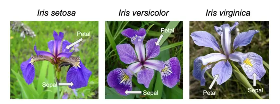
The Iris Dataset contains measurements of a flower’s sepal and petal. There are 50 samples for each of the three species of Iris flowers (150 in total across the Iris setosa, Iris virginica and Iris versicolor species). A sepal is the outer parts of the flower (often green and leaf-like) that enclose a developing bud. The petal are parts of a flower that are the pollen producing part of the flower that are often conspicuously colored. The difference between sepals and petals can be seen below.
For this question, we are interested in estimating the mean petal length for flowers. The unit of measurement for petal length is centimeters. See your data table below.
Data Table
Questions are on the next page
- What R functions were used to calculate the above data table that shows the sample mean and sample standard deviation? Write in the appropriate function for
A1andA2from the list of functions below.
iris |>
  A1(mean_PL = mean(Petal.Length),
sd_PL = A2(Petal.Length))group_by()generate()specify()summarize()aes()se()
A1 = summarize()
A2 = sd()
- Using your data table, report the value of your sample mean. Use proper notation.
\(\bar{x} = 3.758cm\)
- The following questions are going to have you calculate a theory based confidence interval. Use the context of this problem to justify why we are going to calculate a confidence interval, instead of conducting a hypothesis test to answer our research question.
We are creating a confidence interval because the goal of the question is to ESTIMATE.
- Assuming the Central Limit Theorem assumptions are met, what would you expect the shape of the population distribution be of all Iris flower’s petal length?
Normally distributed
Left skewed
Right skewed
(d) Not enough information to answer the question
The CLT does not tell us the shape of the population distribution
- Assuming the Central Limit Theorem assumptions are met, what would you expect the shape of the sampling distribution for the mean petal lengths be?
(a) Normally distributed
Left skewed
Right skewed
Not enough information to answer the question
The CLT suggests that, regardless of the shape of the population distribution, the shape of the sampling distribution for a single mean will be roughly normally distributed if the assumptions are met
- Which code would produce the correct \(t^*\) multiplier used to create a 90% confidence interval? Circle your answer.
qt(.95, df = 149)qt(.90, df = 149)qt(.95, df = 150)qt(.90, df = 150)qt(.95, df = 149); .95 is the quantile to cut off 5% of the tail. df is calculated as n-1
- Using 1.66 as your \(t^*\) multiplier, calculate a 90% confidence interval. Show your work.
\(3.758 \pm 1.66*\frac{1.765}{\sqrt150} = (3.519,3.997)cm\)
- Regardless of your answer part g, assume you calculated the following 90% confidence interval for the population mean petal length (0.758, 6.758). Interpret this confidence interval in the context of the problem.
We are 90% confident that the true mean petal length for iris flowers is between .758 and 6.758 cm.
Question 2 (16 points)
- Recall your 90% confidence interval from question 1: (0.758, 6.758). If you instead calculated a 95% confidence interval, what would change about your interval? Circle all that apply.
- The width of the interval would become narrower
(b) The width of the interval would become wider
The center
The interval remains the same
A 95% confidence interval has a larger multiplier, thus a larger width than a 90% confidence interval.
- Recall your 90% confidence interval from question 1: (0.758, 6.758). If the researchers instead collected a sample size of 100 flowers for each species, what would change about your interval? Assume that everything else stayed the exact same from the study. Circle all that apply.
(a) The width of the interval would become more narrow
The width of the interval would become wider
The center
The interval remains the same
The margin of error is a function of sample size. As n goes up, the standard error goes down… meaning the margin of error goes down… meaning the confidence interval gets more narrow. See \(\frac{s}{\sqrt{n}}\)
- Suppose a different researcher went out and collected a very very large sample of 1000 flowers for each species and calculated a 99% confidence interval: (0.523, 2.489).
What is the value of this new researcher’s sample statistic? Show your work.
The statistic is the center of the interval
\(\frac{2.489 + .523}{2} = 1.506\)
What is the approximate value of this new researcher’s t* multiplier? Justify your answer.
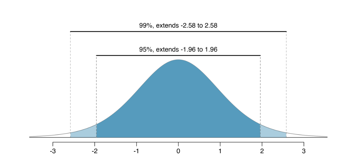
The approximate t multiplier in this scenario is 2.58. This is because a t-distribution with 2999 degrees of freedom is essentially a standard normal distribution, and we know a standard normal distribution uses a multiplier of 2.58 for 99% confidence intervals. 2.58 found on formula sheet
What is the value of this new researcher’s standard error? Show your work.
If you could not approximate the value of the t* multiplier, use may use the value of 2 to help answer this question if needed. If you could not calculate the sample statistic, use may the value of 1 to help answer this question if needed.
\(1.506 + (2.58 x SE) = 2.489\)
\((2.58 x SE) = 0.983\)
\(SE = \frac{0.983}{2.58} = 0.381\)
What is the value of this new researcher’s margin of error? Show your work.
If you could not approximate the value of the t* multiplier, you may use the value of 2 to help answer this question if needed. If you could not calculate the sample statistic, you may use the value of 1 to help answer this question if needed. If you could not calculate the standard error, you may use the value of 5 to answer this question.
The margin of error is the SE multiplied by our t multiplier
ME = 2.58 * .381 = 0.983
Question 3: The Effect of Vitamin C on Tooth Growth in Guinea Pigs (18 points)
The response is the length of odontoblasts (cells responsible for tooth growth) in 60 guinea pigs. This is measured as “High” if the length of odontoblasts was larger than 10mm, and “Small” if the growth was 10mm or less. Each animal received doses of vitamin C either through a vitamin C supplement or by drinking orange juice, which has vitamin C in it.
We are interested in testing if the way the vitamin C was administered is independent from the odontoblasts length. You are researching if the orange juice (OJ) group produces more “High” measurements than the supplement group (VC). You can consider a “success” as a “High” measurement. Use the order of subtraction OJ - VC.
# A tibble: 4 × 3
# Groups:   supp [2]
  supp  measurement count
  <fct> <chr>       <int>
1 OJ    High           23
2 OJ    Low             7
3 VC    High           18
4 VC Low 12- Use the data table above to calculate your sample statistic. Use proper notation.
\(\hat{p}_\text{oj} = \frac{23}{30}\)
\(\hat{p}_\text{vc} = \frac{18}{30}\)
\(\frac{23}{30} - \frac{18}{30} = 0.167\)
- Use the information from the prompt to write out the appropriate null and alternative hypothesis. Use proper notation. You do not need to write this in words, just proper notation.
\(H_o: \pi_\text{oj} - \pi_\text{vc} = 0\)
\(H_a: \pi_\text{oj} - \pi_\text{vc} > 0\)
- Suppose that the Central Limit Theorem assumptions are satisfied. You then conduct a randomization test using a simulated null distribution, which can be seen below.
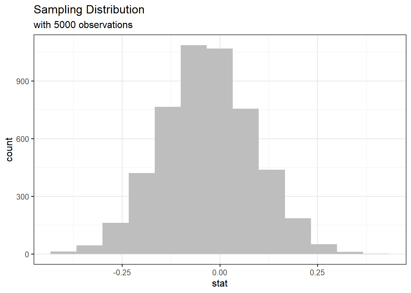
In as much detail as possible, describe how one dot (observation) on this simulated sampling distribution under the assumption of the null hypothesis is created.
– shuffle all 60 observations together, because we assume independence (true proportion of high measurements for the oj group and vc group are the same)
– shuffle observations (sample w/out replacement) into two new groups of size 30 each
– calculate each new sample proportion and subtract
- The corresponding p-value for this test can be seen below.
# A tibble: 1 × 1
  p_value
    <dbl>
1   0.137
Describe how this p-value is calculated (interpret the p-value in the context of the problem).
– probability of observing our statistic of 0.167
– or something even larger
– given the true proportion of high measurements is the same for the OJ and VC group
is about 13.7%
- Write an appropriate decision and conclusion at the \(\alpha = 0.05\) significance level.
We our p-value larger than alpha, we fail to reject the null hypothesis, and have weak evidence to conclude that the true proportion of high measurements for the oj group is larger than the vc group.
- In this question, we assumed that the assumptions for the Central Limit Theorem were satisfied. What are these two assumptions? (I’m not asking you to check them, I’m asking you to name them).
– Success-Failure
(Note: I gave credit to those who said sample size, and sample size > 30… but we should be more specific, and the > 30 rule is not for categorical response variables.)
– Independence
Question 4 (13 points)
Assume that the population distribution of time it takes to get to school for students in a small town in Montana is known and seen below.
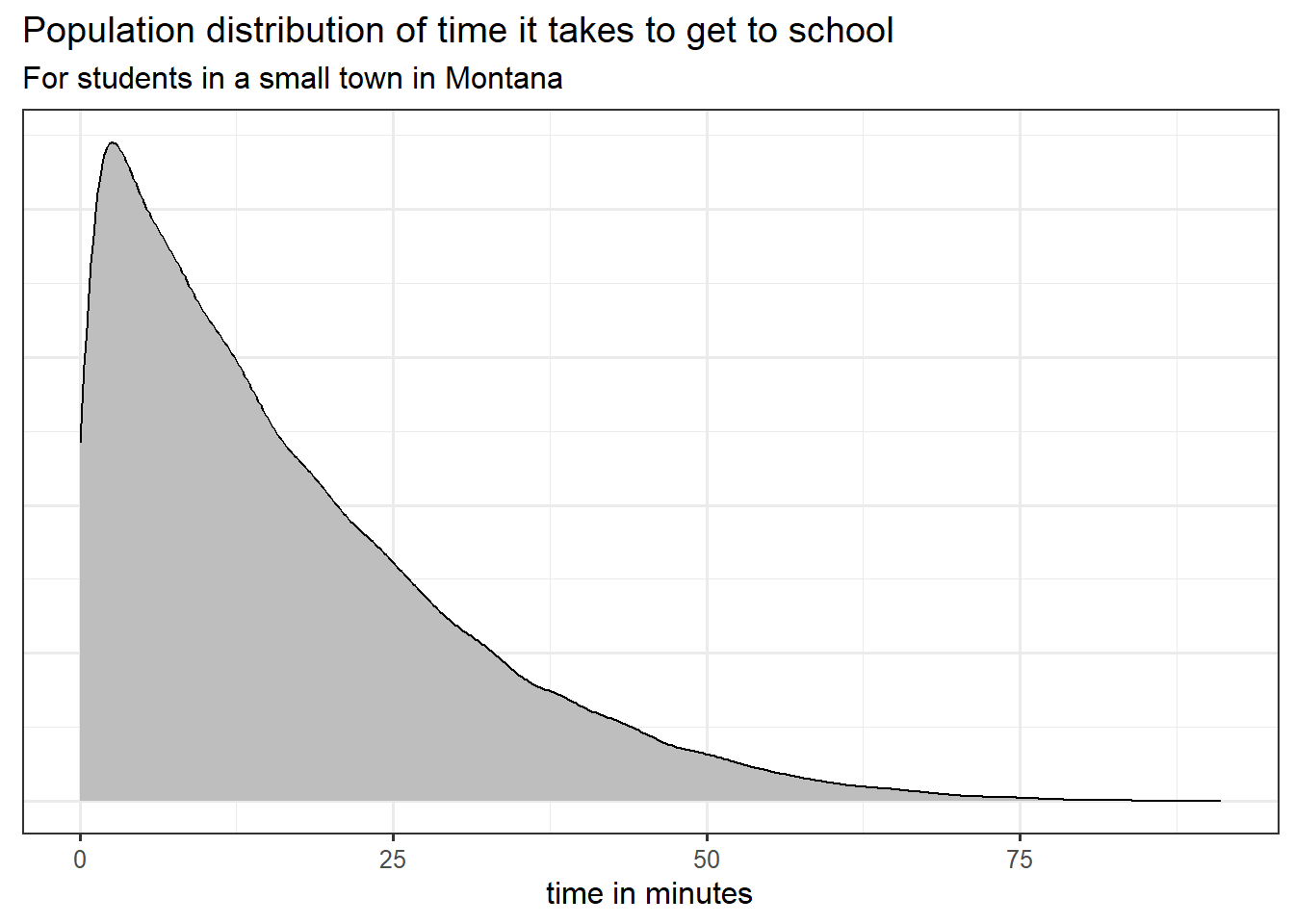
- What is the shape of this population distribution?
(a) Right skewed
Left skewed
Normal
Bimodel
The right tail is longer, making this a right skewed distribution
- Suppose your random variable X is time in minutes. What is the probability that a student takes more than 85 minutes to get to school? Write out the probability statement in proper notation AND report an approximate probability.
P(X > 85) ~ < 0.001..
This is not 0 because we are calculating an area of a region of the distribution… the region is just very very small.
- What is the probability that a student takes exactly 40 minutes to get to school? Justify your answer. Note, you do not have to perform any calculations to answer this question.
P(X = 40) = 0.
The probability of observing a single point on a continuous distribution is equal to 0. There are an infinite amount of values approaching the value of 40 from both sides. Thus, we realize the P(X = 40) to be so small, it is essentially 0 and reported as such.
Standard Normal Distribution Cut Offs
SE Formulas
Single proportion SE calculations
\(\sqrt{\frac{\pi_o * (1-\pi_o)}{n}}\)
\(\sqrt{\frac{\hat{p} * (1-\hat{p})}{n}}\)
Difference in proportions SE calculations
\(\sqrt{\frac{\hat{p_\text{pool}}*(1-\hat{p_\text{pool})}}{n1} + \frac{\hat{p_\text{pool}}*(1-\hat{p_\text{pool})}}{n2}}\)
\(\sqrt{\frac{{\hat{p_1}*(1-\hat{p_1})}}{n_1} + \frac{{\hat{p_2}*(1-\hat{p_2})}}{n_2}}\)
Single mean SE calculations
\(\frac{s}{\sqrt{n}}\)
Difference in means SE calculations
\(\sqrt{{\frac{s_1^2}{n_1}} + \frac{s_2^2}{n_2}}\)
General Confidence Interval Formula
\(statistic \pm multiplier * SE\)
General Formula for Test Statistic
\(\frac{statistic - \text{null value}}{SE}\)
