library(tidyverse)
library(tidymodels)
library(scatterplot3d)
library(palmerpenguins)Additive models
Solutions
Load packages and data
Today
By the end of today you will…
- understand the difference between and additive vs interaction model
- understand the geometric picture of multiple linear regression
- be able to build, fit and interpret linear models with \(>1\) predictor
- think critically about r-squared as a model selection tool
Fitting the additive model
To fit the additive model, we can use the + sign. Use the plus sign to add species to the linear model code fit from Monday’s class.
Call:
lm(formula = flipper_length_mm ~ bill_length_mm + species, data = penguins)

Residuals:
     Min       1Q   Median       3Q      Max
-24.7485  -3.4135  -0.0681   3.6607  15.9965

Coefficients:
                 Estimate Std. Error t value Pr(>|t|)
(Intercept)      147.9511     4.1738  35.447   <2e-16 ***
bill_length_mm     1.0828     0.1069  10.129   <2e-16 ***
speciesChinstrap  -5.0039     1.3698  -3.653    3e-04 ***
speciesGentoo     17.7986     1.1698  15.216   <2e-16 ***
---
Signif. codes:  0 '***' 0.001 '**' 0.01 '*' 0.05 '.' 0.1 ' ' 1

Residual standard error: 5.826 on 338 degrees of freedom
  (2 observations deleted due to missingness)
Multiple R-squared:  0.8299,    Adjusted R-squared:  0.8284
F-statistic: 549.6 on 3 and 338 DF,  p-value: < 2.2e-16
Prediction using R
Let’s use R to make predictions using this additive model. Use R to predict the flipper length for a Gentoo penguin that has a bill length of 60.
predict(model1, data.frame(bill_length_mm = 60, species = "Gentoo"))Interpretation
Now, let’s interpret these coefficients in the context of the problem:
Intercept: For a bill length of 0, we estimate the mean flipper length for the Adelie penguins to be 147.563mm
speciesChinstrap: Holding bill length constant, we estimate the mean flipper length of Chinstrap penguins to be 5.247mm lower than Adelie penguins
bill_length_mm: Holding species constant, for a 1 mm increase in bill length, we estimate the mean flipper length to increase by 1.09mm.
Can we do this with 2 quantitative variables?
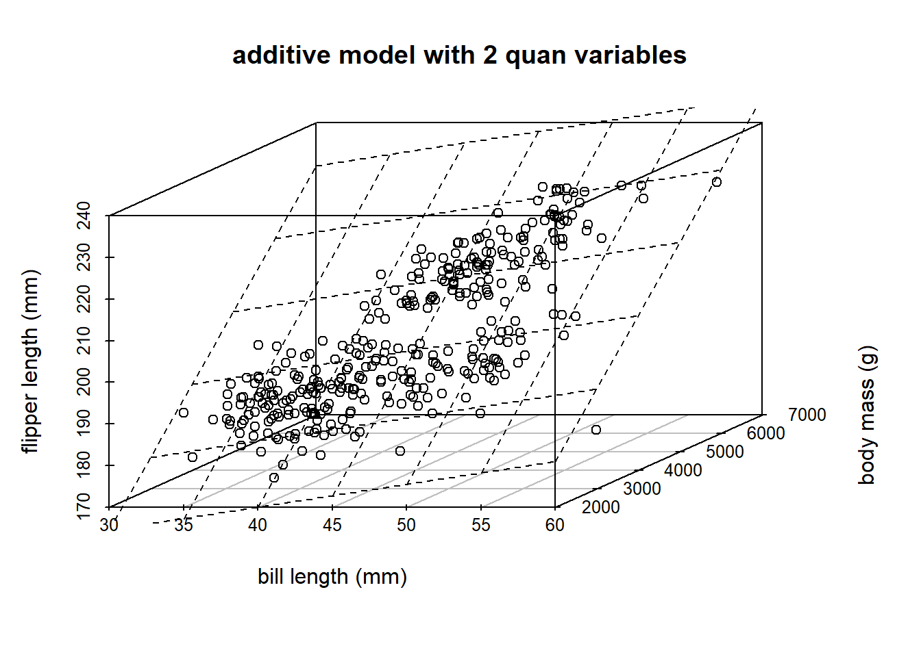
Yes! Let’s look at the explanatory variables bill length (mm) and body mass (g).
The concept is the same, the picture is a bit different! What about, instead of species, we wanted to use body_mass_g. Note, the following code is to help us understand the material, and is not a learning objective of the course. The code you need to know is lm.
s3d <- penguins |>
  dplyr::select(bill_length_mm, body_mass_g, flipper_length_mm) |>
  scatterplot3d(xlab = "bill length (mm)",
                ylab = "body mass (g)",
                zlab = "flipper length (mm)",
                main = "additive model with 2 quan variables")
Warning: Unknown or uninitialised column: `color`.model2 <- lm(flipper_length_mm ~ bill_length_mm + body_mass_g, penguins)
s3d$plane3d(model2)
               Estimate Std. Error t value Pr(>|t|)
(Intercept)     121.956      2.855  42.715        0
bill_length_mm    0.549      0.080   6.859        0
body_mass_g       0.013      0.001  23.939        0