Introduction to Simulation Testing + Confidence Inverals
Lecture 9
NC State University
ST 511 - Fall 2024
2024-09-18
Checklist
– Keep up with Slack
– Quiz-4 comes out today (5:00pm)
– HW-2 is out (due Monday 23rd)
– HW-1 Solutions are out
– HW-1 grades coming soon (working with TAs)
– Run install.packages("tidymodels") in your Console for today’s activity
Announcement
LaTeX Code
LaTeX is not a requirement for this course. If you want the opportunity to build up this skill, please do so.
\(\mu\) = mu
\(\pi\) = pi
\(\hat{p}\) = p-hat
\(H_o\) = Ho
The list goes on….
Warm Up Questions
Suppose we are interested in penguin species on an island in Palmer Archipelago. We know that there are three species of penguins (Adelie, Chinstrap, Gentoo) on this island. It is assumed that there is an even distribution of all three species of penguins. We think that the Gentoo species has become more dominant, and there are more of this species than assumed.
What is our population parameter in words? What are our null and alternative hypotheses?
\(H_o:\)
\(H_a:\)
Warm Up Questions
Suppose we are interested in penguin species on an island in Palmer Archipelago. We know that there are three species of penguins (Adelie, Chinstrap, Gentoo) on this island. It is assumed that there is an even distribution of all three species of penguins. We think that the Gentoo species has become more dominant, and there are more of this species than assumed.
\(\pi\) = The true proportion of Gentoo penguins on an island in Palmer Archipelago.
\(H_o:\) \(\pi\) = .33
\(H_a:\) \(\pi\) > .33
Warm Up Question
Let’s assume that your test statistic (Z-statistic) for this penguin study was 5.78. Use pnorm to calculate your p-value.
- Let’s talk why you are getting the answer you are!
Recap of last time
– Set up our null and alternative hypotheses
– Collected data and calculated our sample statistic
– Approximated or standardized our statistic to follow a named distribution
– Calculate p-value
– Write decision; conclusion; and interpretation
Approximate / Standardize
Howling Cow Example
\(H_o:\) \(\pi\) = .5
\(H_a:\) \(\pi\) < .5
\(\hat{p}\) = \(\frac{37}{100}\)
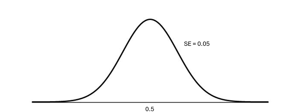
Our entire goal is to make a null distribution! This distribution is:
– centered at \(\pi_o\)
– has spread (standard error for the null) of
\[ \sqrt{\frac{.5 * (1-.5)}{100}} \]
It has this standard error because we checked our assumptions!
What’s this look like
Here is the approximated null distribution. And we can calculate the p-value straight from here!
Standardized Statistic
Why?
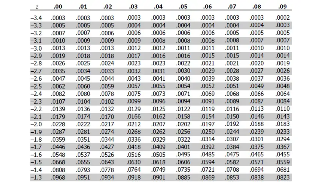
Before technology, a bunch of people did some really hard calculus, so the probabilities of a standard normal distribution were known.
Standardized Statistic
Why today?
– It helps us compare Z-scores across studies (has no units)
– It’s a common practice most fields still use
Z = \(\frac{\hat{p} - \pi_o}{SE}\)
Z = \(\frac{.37 - .5}{0.05}\) = -2.61
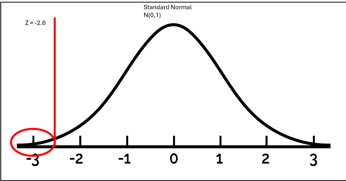
Theory vs Simulation
The null distribution can be estimated through simulation (simulation-based methods), or can be modeled by a mathematical function (theory-based methods)
Let’s now talk about simulation (and practice with it in R)
Simulation
– Simulation studies started to become popular as technology advanced
– Still need an independence assumption
– Less strict sample size assumption. Simulation studies can be used with smaller sample sizes than traditional statistical methods, but it may not be effective for very small samples. Although there isn’t a strict cut-off, some suggest
  - Typically > 5 success + failures (categorical)

  - sample size > 15 (quantitative)
sep-18-ae
Bumba vs Kiki
