# A tibble: 1 × 1
   corr
  <dbl>
1 0.656Regression II
Lecture: ???
NC State University
ST 511 - Fall 2024
2024-11-04
Checklist
– Keep up with Slack; I’m giving advice on HW-4
– Take-home key is posted. Take a look (not during class..)
– HW 4 (due Sunday Nov 10)
– Quiz 9 (released Wednesday; due Sunday Nov 10)
– Download today’s AE
Announcements
Help files are important! cor is a little different than our typical functions…
Warm Up Question
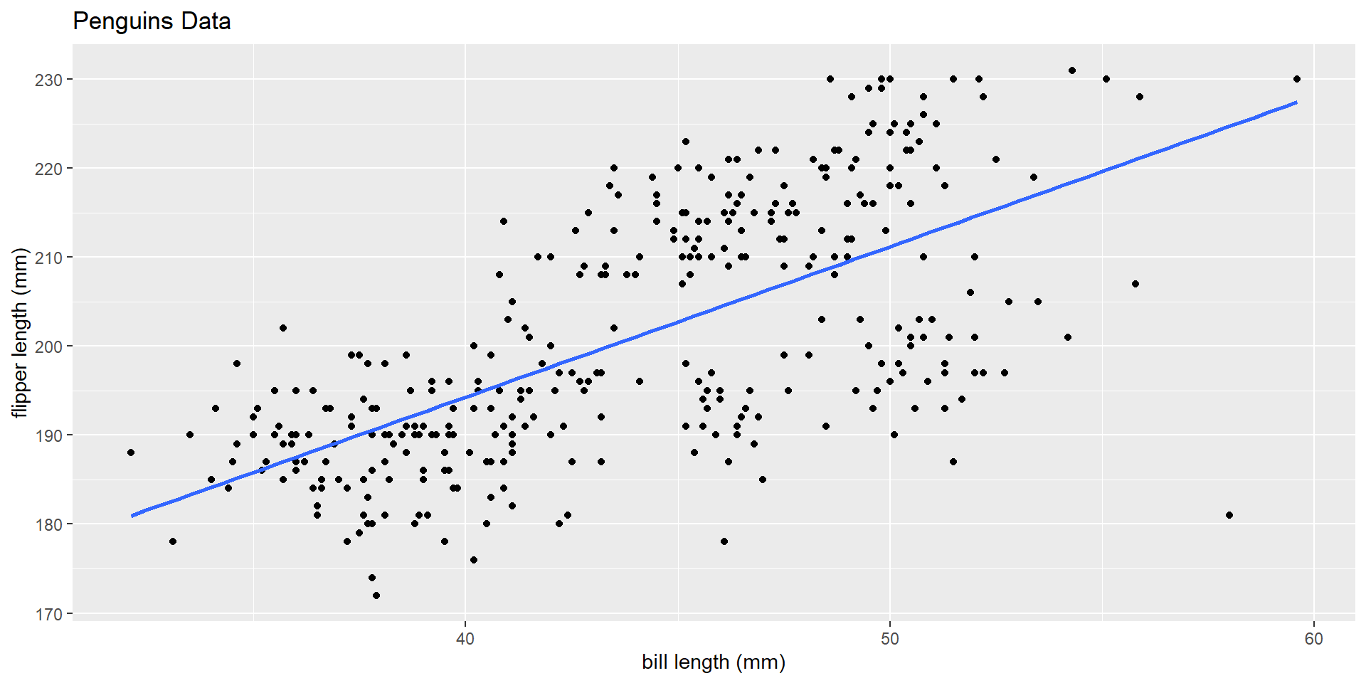
Last time, we set the stange to be interested in looking at the relationship between flipper length and bill length. Specifically, we were interested bill length’s impact on flipper length. We fit a line to understand this realtionship. How was this line fit?

Warm Up Question
\(e_i = y - \hat{y}\)
where y is an observed value, and \(\hat{y}\) is the predicted value based on the line!
Minimize the residual sums of squares: \(\sum (y_i - \hat{y_i})^2\)
In R
Warm Up Question
What can do with this line?

Warm Up Question
What can do with this line?
– Prediction
– Interpretations
– Hypothesis testing (see Ch. 24 and on!)
The line
\(\widehat{\text{flipper length}} = 126.68 + 1.69*\text{bill length}\)
How can we interpret the slope?
How can we interpret the intercept?
Interpretations
Slope: For a 1 mm increase in bill length, we estimate on average, a 1.69 mm increase in flipper length.
Intercept: We estimate a mean flipper length of 126.68 mm for a penguin that has a bill length of 0 mm.
Prediction
How can we use the following line to make predictions about mean flipper length?
\(\widehat{\text{flipper length}} = 126.68 + 1.69*\text{bill length}\)
Prediction
Do you have any concerns about predicting bill length at 50? 60? 150?
\(\widehat{\text{flipper length}} = 126.68 + 1.69*\text{bill length}\)

Prediction
That uneasy feeling = extrapolation!
We do not know how the data outside of our limited window will behave, but this model is going to assume a linear relationship between bill length and flipper length!
Strength of fit
We evaluated the strength of the linear relationship between two variables earlier using the correlation. Another (more common and flexible) summary statistic is called R-Squared (\(R^2\)).
This is also called the coefficient of determination
\(R^2\) of a linear model describes the amount of variation in the response variable, that is explained by our explanatory variable.
R-Squared
\[ R^2 = \frac{SST - SSE}{SST} \]
We’ve seen this idea before…
R-Squared
\(SST = \sum (y_i - \bar{y})\)
\(SSE = \sum (y_i - \hat{y_i})^2\)
R-Squared
\(SST = \sum (y_i - \bar{y})\)
\(SSE = \sum (y_i - \hat{y_i})^2\)

R-Squared
For simple linear regression..
\((r)^2 = R^2\)
We can square the correlation coefficient to get the coefficient of determination (R-squared)
R-Squared calculation
R-Squared calculation
Questions
Should we consider other variables?
Do we think that bill length is the only explanatory variable we should use to under flipper length?
What others might be good?
Should we consider other variables?
Do we think the relationship between bill length and flipper length depends on the species of penguin? Let’s investigate!
AE
Model Output
\(\widehat{\text{flipper length}} = 147.563 + 1.10*\text{bill length} -\) \(5.25*\text{Chinstrap} + 17.55*\text{Gentoo}\)
\[\begin{cases} 1 & \text{if Chinstrap level}\\ 0 & \text{else} \end{cases}\] \[\begin{cases} 1 & \text{if Gentoo level}\\ 0 & \text{else} \end{cases}\]