# A tibble: 1 × 1
corr
<dbl>
1 0.656Regression
Lecture: ???
NC State University
ST 511 - Fall 2024
2024-11-04
Checklist
– Are you keeping up with Slack?
– Are you keeping up with the prepare material?
– HW 4 (released today; due Sunday Nov 10)
> Recreating r-code output
> chi-square
– Quiz 9 (released Wednesday; due Sunday Nov 10)
Announcements
Late window for HW-3 (due by tonight at 11:59pm); 10% deduction
Note: I won’t take off 10% for your exam corrections as well; just the HW
Announcements
The take-home exam is graded; thank you for your patience
> median: 87.3%; mean: 83.6%; max: 99%A lot of work went into these. I’m very impressed with how far the class has come with both the methodology + coding
Grades will be published sometime this afternoon. Key will also be up on our website (don’t share it…)
Updating Grades
If you submit a regrade request, and you see your grade changed on Gradescope… you will NOT see your grade changed on Moodle until we re-sync grades. I do this about three times a semester (once after exam-1 is done, and again closer to the final, and once at the very end of the semester)
Announcements
We’ve been using the wrong WorkBench link…
Should be using: https://rstudio.stat.ncsu.edu/
A couple of you are running into a “rate limit” which is preventing you from using the WorkBench. This is because the link we are using isn’t running through the NCSU servers like we should be.
Suggestion
– I would start using https://rstudio.stat.ncsu.edu/
– Your previous work won’t be there, but you can move it over
– Will prevent you from getting locked out of WorkBench due to rate limit
– This link can also be found on our website/moodle/ etc.
Announcements
As posted on Slack
Office hours are moving from Monday to Thursday: 10:30 - 11:30am
> This is so you can take advantage of OH for HW-4 and Quiz-9
> This move will be for the rest of the semester
> This has been updated on our website
Question? Comments?
Learning objectives
– Understand how to summarize two quantitative variables
– What is simple linear regression (SLR)?
– How a line of best fit is made
– How to talk about the line of best fit
SLR
Suppose now I wanted to investigate the relationship between bill length and flipper length.
– Can I analyze these data using difference in means?
– Difference in proportions?
What plot could we use to look at these data?
Plot the data
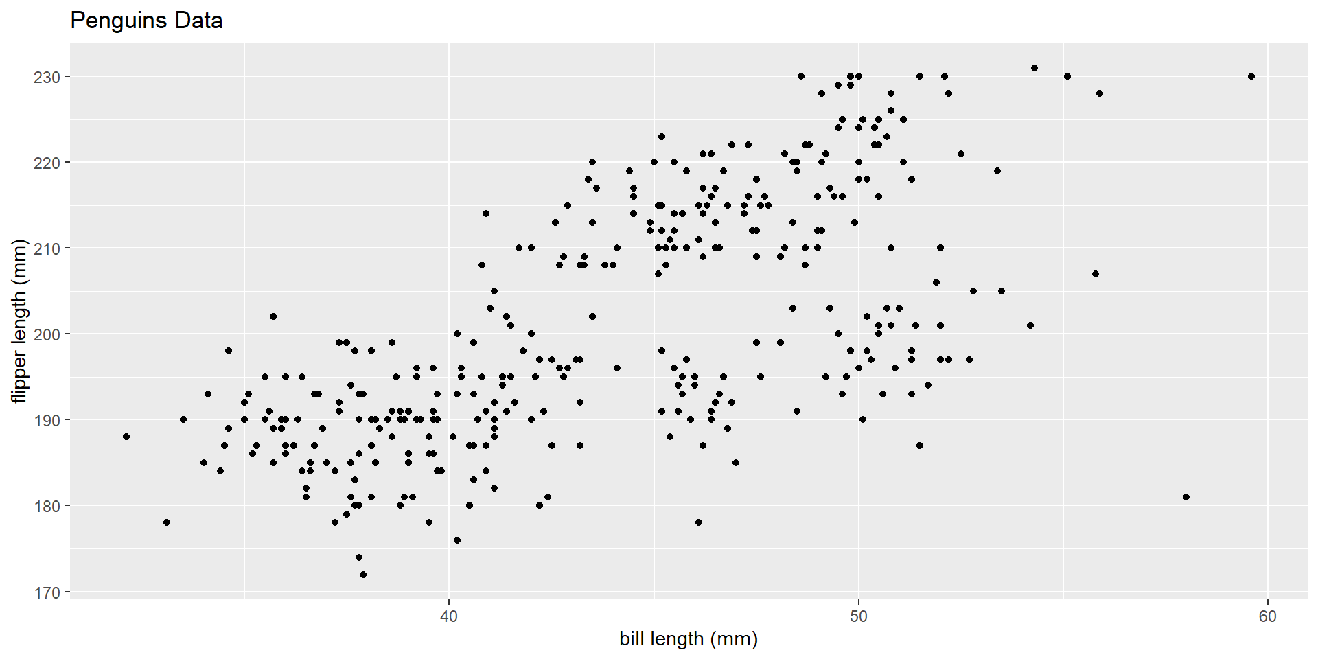
How can we summarize these data?
Summary statistics
– correlation (r)
– slope + intercept (fit a line)
Correlation
– Is bounded between [-1, 1]
– Measures the strength + direction of a linear relationship
What do I mean by linear relationship?
What do I mean by strength?
What do I mean by direction?
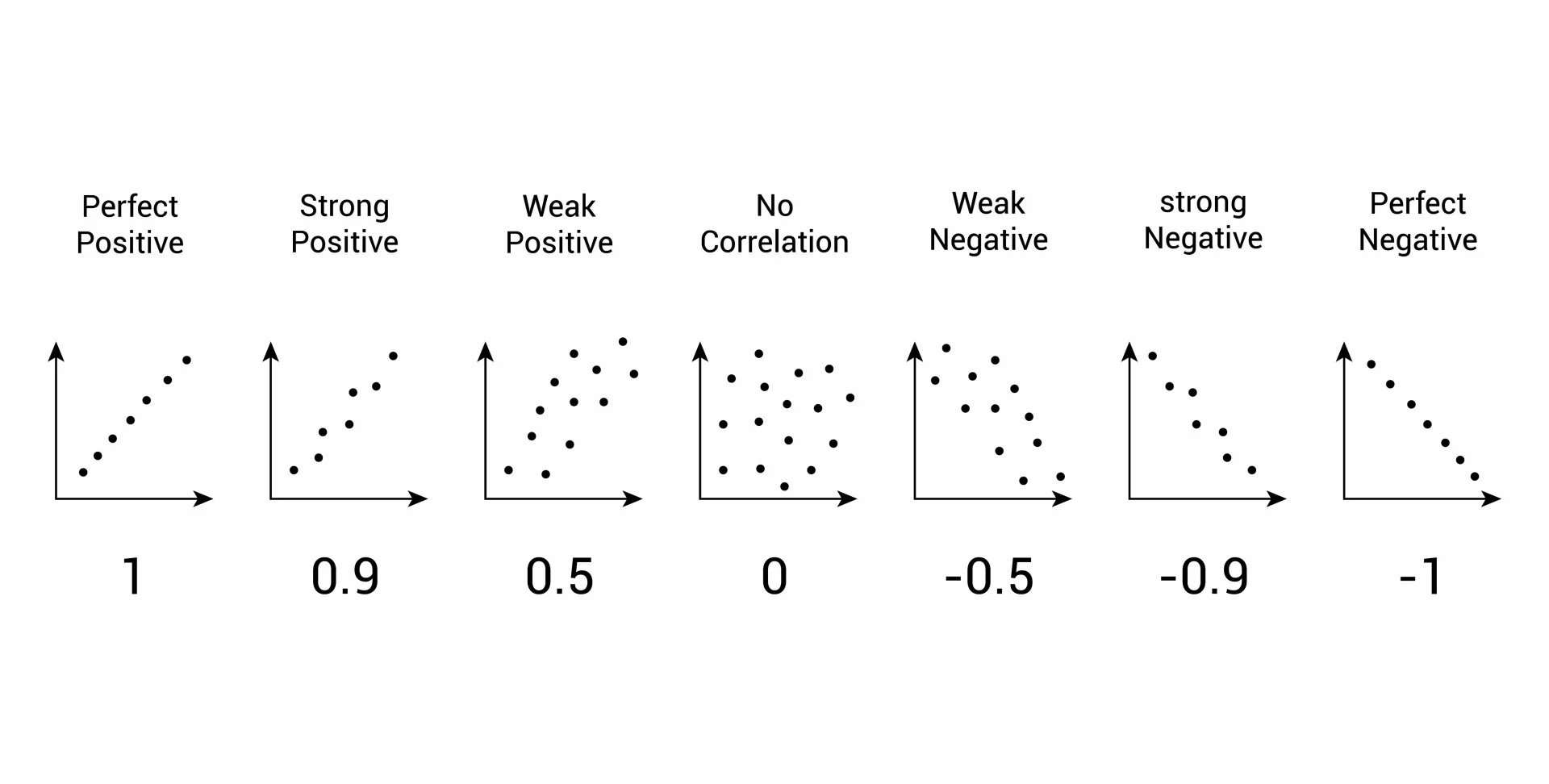
Guessing Game

Let’s find the correlation coefficient between our two variables
syntax: cor(x, y)
Summary statistics
– correlation (r) ✔️
– slope + intercept (fit a line)
Fit a line
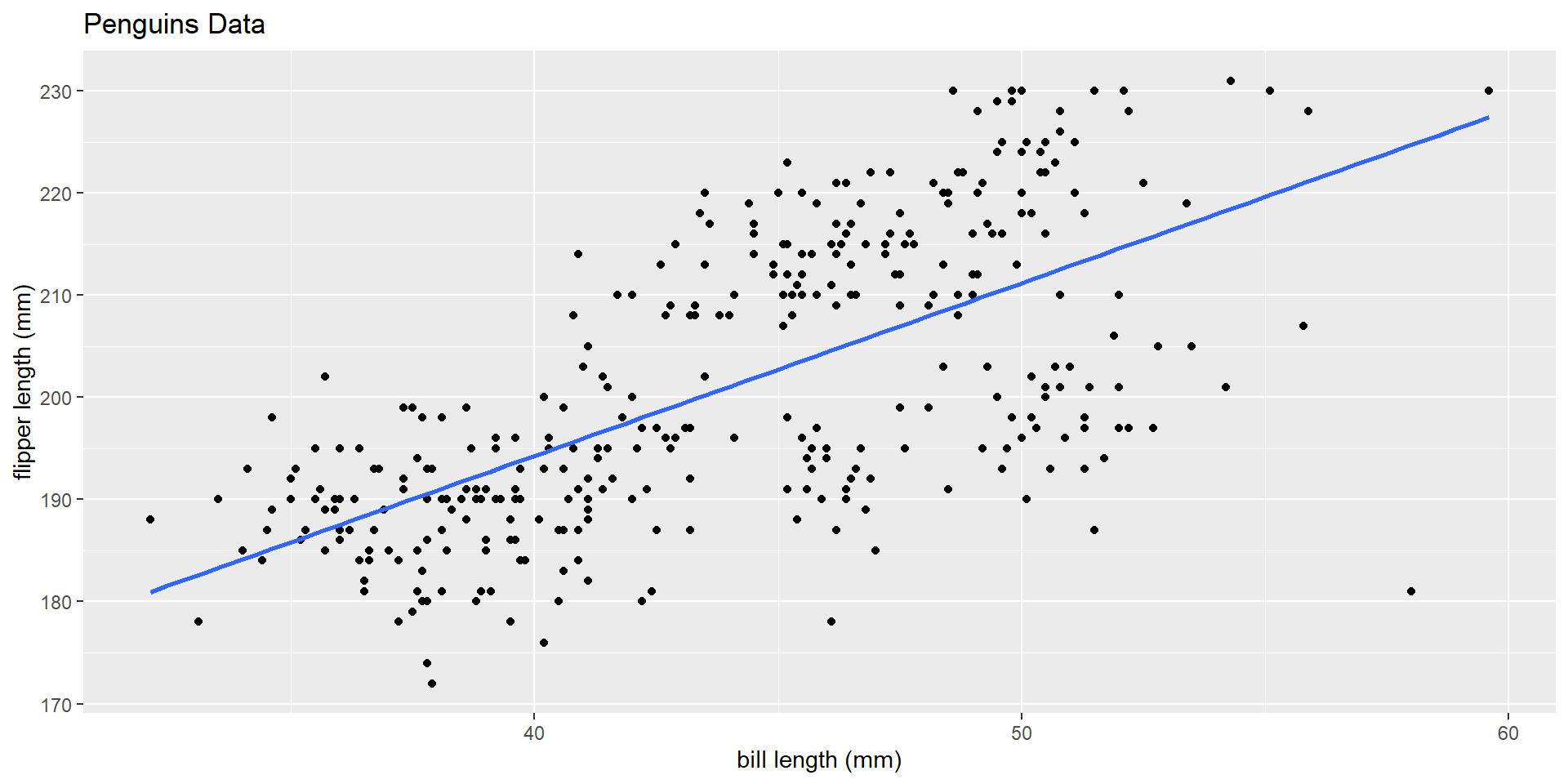
How do we suppose that this line was fit?
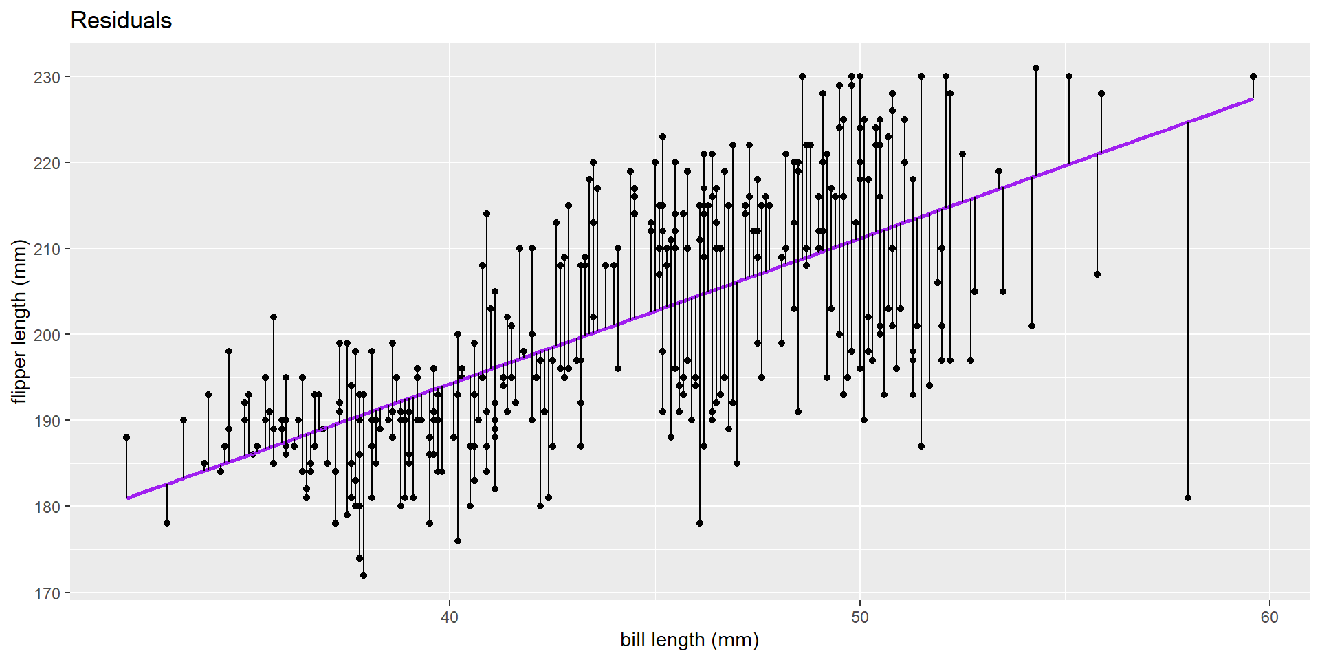
Residual
\(e_i = y - \hat{y}\)
where y is an observed value, and \(\hat{y}\) is the predicted value based on the line!
Minimize the residual sums of squares: \(\sum (y_i - \hat{y_i})^2\)
Residual
What can we do with this line?
Why do you suppose we fit a line?
– Prediction
– Interpretation
– Hypothesis testing to test for a relationship (May or may not cover in class; I’ll post readings)
The equation
Have you heard of \(y = mx + b\) ?
The equation
Let me introduce you to:
Population level: \(y = \beta_o + \beta_1*x + \epsilon\)
Sample: \(\hat{y} = \hat{\beta_o} + \hat{\beta_1}*x\)
The equation
\(\hat{y}\) (yhat) = predicted value of y
\(\hat{\beta_o}\) (b) = estimated intercept
\(\hat{\beta_1}\) (b1) = estimated slope
\(x\) = explanatory variable
Terms
– What is an intercept?
– What is a slope coefficient?
In-R
Call:
lm(formula = flipper_length_mm ~ bill_length_mm, data = penguins)

Residuals:
    Min      1Q  Median      3Q     Max
-43.708  -7.896   0.664   8.650  21.179

Coefficients:
               Estimate Std. Error t value Pr(>|t|)
(Intercept)    126.6844     4.6651   27.16   <2e-16 ***
bill_length_mm   1.6901     0.1054   16.03   <2e-16 ***
---
Signif. codes:  0 '***' 0.001 '**' 0.01 '*' 0.05 '.' 0.1 ' ' 1

Residual standard error: 10.63 on 340 degrees of freedom
  (2 observations deleted due to missingness)
Multiple R-squared:  0.4306,    Adjusted R-squared:  0.4289
F-statistic: 257.1 on 1 and 340 DF,  p-value: < 2.2e-16
Writing out our model
\(\hat{y} = \hat{\beta_o} + \hat{\beta_1}*x\)
\(\widehat{\text{flipper length}} = 126.68 + 1.69*\text{bill length}\)
How do we interpret the intercept? How do we interpret the slope coefficient?
Slope coefficient
bill length of 1
\(\widehat{\text{flipper length}} = 126.68 + 1.69*\text{bill length}\)
\(\widehat{\text{flipper length}} = 126.68 + 1.69*1\)
\(\widehat{\text{flipper length}} = 128.37\)
Slope coefficient
bill length of 2
\(\widehat{\text{flipper length}} = 126.68 + 1.69*2\)
\(\widehat{\text{flipper length}} = 126.68 + 3.38\)
\(\widehat{\text{flipper length}} = 130.06\)
130.06 - 128.37 = 1.69 (The amount we move up as bill length increased by 1 mm)
Interpretation
For a 1 mm increase in bill length we estimate a 1.69 mm increase in mean flipper length
For a 1 mm increase in bill length, we estimate on average, a 1.69 mm increase in flipper length.
Why mean flipper length?
We are estimating the mean flipper length, because our model is calculating the expected value of flipper length at a given bill length.
Why mean flipper length?
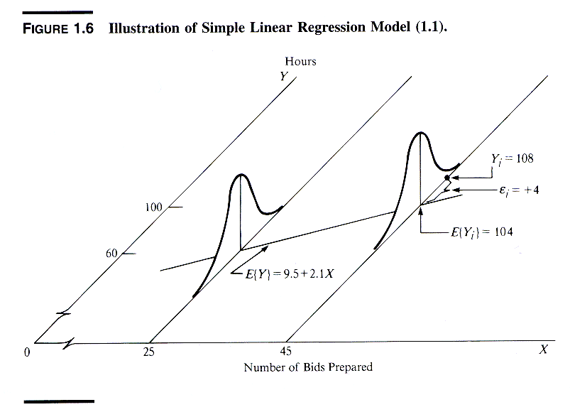
The phrase expected value is a synonym for mean value in the long run (meaning for many repeats or a large sample size).
Intercept
\(\widehat{\text{flipper length}} = 126.68 + 1.69*\text{bill length}\)
\(\widehat{\text{flipper length}} = 126.68 + 1.69*0\)
\(\widehat{\text{flipper length}} = 126.68 + 0\)
\(\widehat{\text{flipper length}} = 126.68\)
We \(\widehat{estimate}\) a mean flipper length of 126.68 mm for a penguin that has a bill length of 0 mm.
Prediction
How would we use this line for prediction? What would we predict a penguin’s flipper length to be if a penguin had a bill length of 50mm?
Prediction
\(\widehat{\text{flipper length}} = 126.68 + 1.69*\text{bill length}\)
\(\widehat{\text{flipper length}} = 126.68 + 1.69*50\)
== 211.18mm
We would predict a penguin with a bill length of 50 mm to have an average flipper length of 211.18 mm.
