Logistic Regression
Lecture: ???
NC State University
ST 511 - Fall 2024
2024-11-18
Checklist
– Keep up with Slack
– HW 5 (due Tuesday at 11:59)
– HW 6 has been released (due Tue 26th at 11:59; our last HW!)
– Quiz 11 (released Wednesday; due Sunday Nov 24)
– Don’t forget about the statistics experience (Due Dec 6th)
Announcements
Office Hour change
– Tuesday (11/19) now from 2:30 - 3:30pm (just for this week)
Warm Up
Anova vs Chi-Square
– When can we use each?
– What is the test statistic for each?
– What distribution does each test statistic follow?
Anova
– Extension of difference in means
– \(Ho: \mu_1 = \mu_2 = \mu_3 = ... \mu_k\)
– \(Ha: \text{At least one population mean is different}\)
– F-statistic ~ \(F_\text{k-1, n-k}\)
Chi-square
– This is a test of independence between categorical data with any number of levels
– \(Ho: \text{x and y are independent}\)
– \(Ha: \text{x and y are not independent}\)
– chi-squared statistic \((\chi^2)\) ~ chi-square distribution \(\chi^2_\text{(r-1)*(c-1)}\)
Roadmap
– In unit 1 + Anova & Chi-square, we have done inferential statistics (taking a sample, and making claims about a larger population)
– In unit 2, we have used regression tools more descriptively (using data to make predictions, and interpret coefficients estimated from our data)
New topics:
– Logistic Regression
– Sampling methods
Goal
Gain some exposure to logistic regression
We can’t learn everything in a week, but we can start to build a foundation
Goal
– The What, Why, and How of Logistic Regression
– How to fit these types of models in R
– How to calculate probabilities using these models
What is Logistic Regreesion
Similar to linear regression…. but
Modeling tool when our response is categorical
AE for motivation
What we will do today
– This type of model is called a generalized linear model
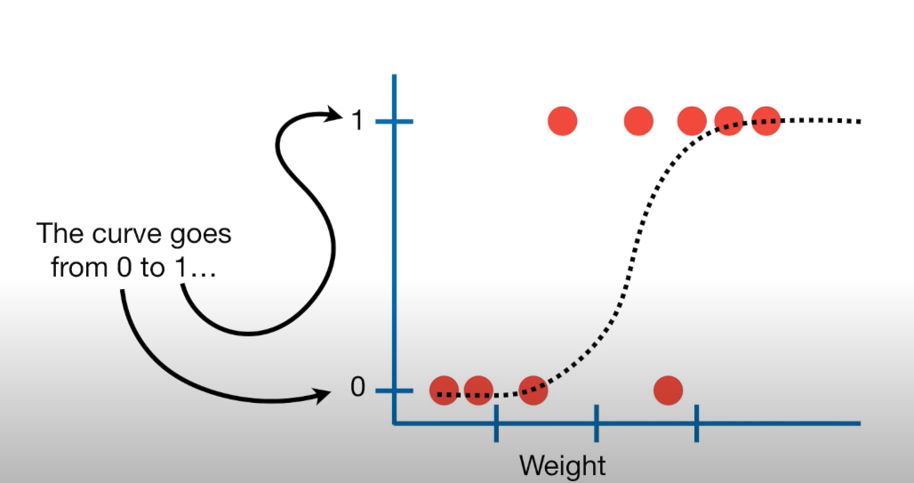
We want to fit an S curve (and not a straight line)…
where we model the probability of success as a function of explanatory a variable(s)
Terms
– Bernoulli Distribution
2 outcomes: Success (p) or Failure (1-p)
\(y_i\) ~ Bern(p)
What we can do is we can use our explanatory variable(s) to model p
Note: We use \(p_i\) for estimated probabilities
Probability
What values can probability take on?
Probability
Probabilities can take on the values of [0,1]…
Need: this means that we need to work with a model that constrains estimated probabilities (our response) to be on the correct scale [0,1]
The S curve
We can accomplish this using the following model

\(\widehat{ln(\frac{p}{1-p}})\) = \(\widehat{\beta_o} +\widehat{\beta}_1X1 + ....\)
Breaking down the model
\(ln(\frac{p}{1-p})\) is called the logit link function, and can take on the values from \(-\infty\) to \(\infty\)
\(ln(\frac{p}{1-p})\) represents the log odds of a success
p stands for probability
This logit link function restricts p to be between the values of [0,1]
Which is exactly what we want!
Breaking down the model
\(\widehat{ln(\frac{p}{1-p}}) = \widehat{\beta_o} +\widehat{\beta}_1X1 + ....\)
These are the coefficients that help us estimate the log odds, conditional on explanatory variable(s) in the model
The S curve

\(\widehat{ln(\frac{p}{1-p}}) = \widehat{\beta_o} +\widehat{\beta}_1X1 + ....\)
Currently, this model is modeling log odds… let’s go through and math out the model we need to use in order to estimate probabilities!
Math
\(\widehat{ln(\frac{p}{1-p}})\) = \(\widehat{\beta_o} +\widehat{\beta}_1X1 + ....\)
– How do we take the inverse of a natural log?
– Taking the inverse of the logit function will map arbitrary real values back to the range [0, 1]
So
\[\widehat{ln(\frac{p}{1-p}}) = \widehat{\beta_o} +\widehat{\beta}_1X1 + ....\]
– Lets take the inverse of the logit function
– Demo Together
Final Model
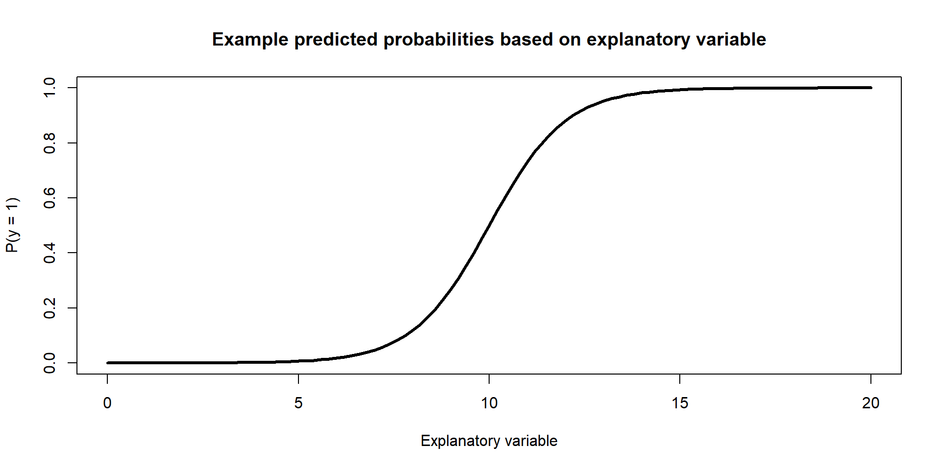
\[\hat{p} = \frac{e^{\widehat{\beta_o} + \widehat{\beta_1}X1 + ...}}{1 + e^{\widehat{\beta_o} + \widehat{\beta_1}X1 + ...}}\]
Example Figure:
Recap
With a categorical response variable, we use the logit link (logistic function) to calculate the log odds of a success
\(\widehat{ln(\frac{p}{1-p})}\) = \(\widehat{\beta_o} +\widehat{\beta}_1X1 + ....\)
We can use the same model to estimate the probability of a success
\[\hat{p} = \frac{e^{\widehat{\beta_o} + \widehat{\beta_1}X1 + ...}}{1 + e^{\widehat{\beta_o} + \widehat{\beta_1}X1 + ...}}\]
AE
Takeaways
– We can not model these data using the tools we currently have
– We can overcome some of the shortcoming of regression by fitting a generalized linear regression model
– We can model binary data using an inverse logit function to model probabilities of success
