# A tibble: 3 × 2
species count
<fct> <int>
1 Adelie 152
2 Chinstrap 68
3 Gentoo 124Anova
Lecture ?
NC State University
ST 511 - Fall 2024
2024-10-16
Checklist
– Take-home exam due Friday (11:59pm)
– Keep up with exam-1 Slack
– No quiz this week
– No hw this week
Announcements
– I’ll have the in-class graded by Friday afternoon (Sunday by the latest)
– I’ll make an announcement on exam corrections once I see the grade distribution
> Won't be the entire exam (1 or 2 questions)
Wrap up unit 1: review
Suppose you calculate a p-value of -0.147. From this, you can determine that…
– You have an observed statistic that is really unlikely to be observed under the assumption of the null hypothesis
– You made some arithmetic mistake. P-values can not be negative
– Your test statistic is negative
– Every value in your data set is negative
Wrap up unit 1: review
Suppose a researcher, using a t-distribution with 20 degrees of freedom, calculated a p-value to be 0.076. Assuming that everything else regarding the study stayed exactly the same, what would happen to the p-value if we used a t-distribution with 5 degrees of freedom…
– The p-value would be larger
– The p-value would be smaller
– The p-value would stay exactly the same
Wrap up unit 1: review
Assuming the Central Limit Theorem assumptions are met, what would you expect the shape of the population distribution be of all Iris flower’s petal length?
– Normally distributed
– Left skewed
– Right skewed
– Not enough information to answer the question
Wrap up unit 1: review
Regardless of your answer part g, assume you calculated the following 90% confidence interval for the population mean petal length (0.758, 6.758). Interpret this confidence interval in the context of the problem.
New Content
Inference on many means
We will use the penguins data set for the slides example, and practice with a new data set for an AE example (Monday).
Inference on many means
In our last example, species impact on bill length. We limited our question to Gentoo and Chinstrap penguins. How species or penguin are in the data set?
Anova
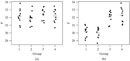
Analysis of variance (ANOVA) is used to test whether the mean outcome differs across two or more groups.
ANOVA uses a test statistic, the F-statistic, which represents a standardized ratio of variability in the sample means relative to the variability within the groups.
The Big Idea

The Big Idea

Theory based
If we assume \(H_o\) is true and the model conditions are satisfied, an F-statistic follows an F-distribution.
What is \(H_o\)?
What are our model conditions?
What is a F-distribution?
Null hypothesis
What is our null hypothesis if we want to test if at least one true mean bill length is different across the three species of penguin? What’s the proper notation for it?
Null hypothesis
\(\mu_g = \mu_c = \mu_a\)
Theory based
If \(H_o\) is true and the model conditions are satisfied, an F-statistic follows an F-distribution.
– What is \(H_o\)? ✔️
– What are our model conditions?
– What is a F-distribution?
Model conditions
Independence
Normality
Constant Variance
Independence
Within and between groups
  > Do we have a random sample?
  > Is there an obvious reason why observatiosn are dependent on each other (ex. space and time)?
Normality

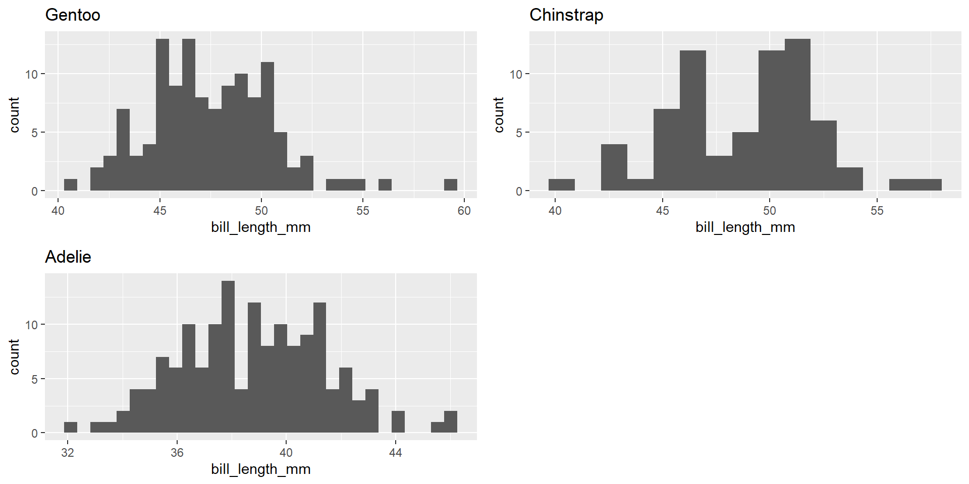
Normality
Outliers?

Sample size
Constant Variance
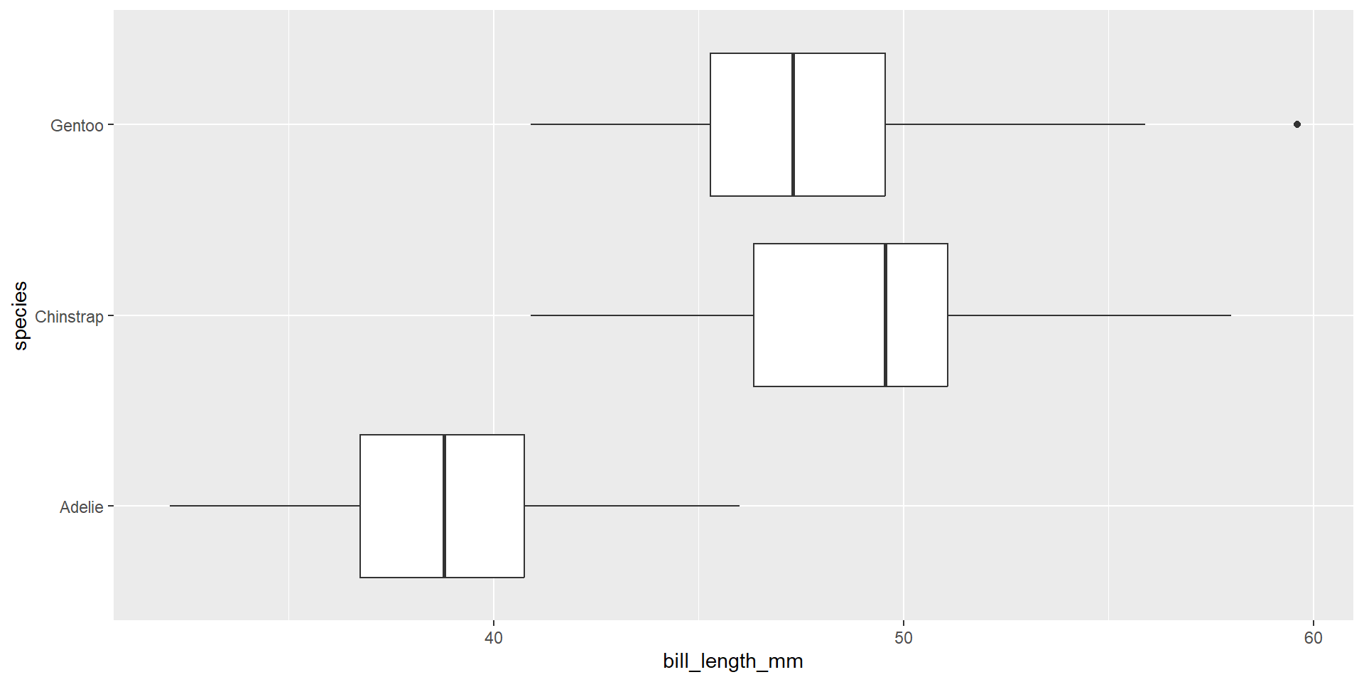
Are the spreads within each group about the same? The constant variance condition is especially important when the sample sizes differ between groups

Rule of thumb
To check for equal variances, you can compare the smallest and largest sample standard deviations. A rule of thumb is that the ratio of the largest and smallest sample standard deviations should not exceed 2.
Rule of thumb
– Some fields use 3
– Levene test
– Welch one-way test
– Residual vs Fitted plot (we will talk about these types of plots when we get to fitting models)
Theory based
If \(H_o\) is true and the model conditions are satisfied, an F-statistic follows an F-distribution.
– What is \(H_o\)? ✔️
– What are our model conditions? ✔️
– What is a F-distribution?
F-Distribution
– The curve is not symmetrical but skewed to the right.
– There is a different curve for each set of degrees of freedom
– We have two sets of degrees of freedom (df) to estimate
  > One for the mean square between groups (k-1) where k is the number of groups (numerator df)
  > One for the mean square error (n-k) where n is the total sample size (denomanator df)
– F-statistics can not be negative
Degrees of freedom
Generally, degrees of freedom is equal to the number observations we use to estimate parameters minus the number of parameters we are trying to estimate
I like to think about degrees of freedom as cogs that shape our theoretical distribution based on our observations
Question What are the numerator and denominator degrees of freedom for our penguin study? Hint: our sample size is 342
Degrees of freedom
We have 3 groups (k)
Numerator df = 3 - 1 = 2
We have 342 - 3 = 339
Theory based
If \(H_o\) is true and the model conditions are satisfied, an F-statistic follows an F-distribution.
– What is \(H_o\)? ✔️
– What are our model conditions? ✔️
– What is a F-distribution? ✔️
Alternative hypothesis
\(H_a\) At least one population mean bill length is different
In R
# Compute the analysis of variance
res.aov <- aov(bill_length_mm ~ species, data = penguins)
# Summary of the analysis
summary(res.aov)
Df Sum Sq Mean Sq F value Pr(>F)
species 2 7194 3597 410.6 <2e-16 ***
Residuals 339 2970 9
---
Signif. codes: 0 '***' 0.001 '**' 0.01 '*' 0.05 '.' 0.1 ' ' 1
2 observations deleted due to missingness