Single Mean Hypothesis Testing
Lecture 12
NC State University
ST 511 - Fall 2024
2024-09-30
Checklist
– Are you keeping up with Slack?
– Quiz-6 Wednesday (due Sunday)
– Exam-1: October 9th (in-class)
– Exam-1: Assigned October 9th; Due 11:59pm October 15th
– Extra credit is live!
Extra credit
Extra credit opportunity: Prepare material for Wednesday (Oct-2nd)
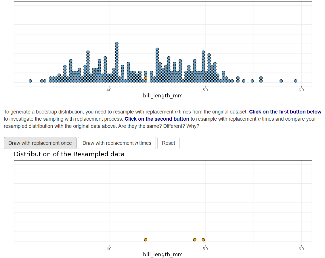
5-10 minute survey Qualtrics survey on if this applet helped!
No id questions at the end; Qualtrics has id information and/or I’ll ask for it
Exam-1 in-class
– You will not do live coding during the exam
– Please bring a calculator
– Closed book + closed notes
– You will be provided formula sheet (check website Wednesday)
Exam-1 in-class (15% of grade)
– Potential coding questions
- ggplot(); group_by(); summarize(); etc
– Multiple choice questions; short answer questions
– Extension question(s)
- demonstrate understanding of fundemental concepts in "new" way
Example
Exercise 5 - HW2
Example
\(\hat{p} \pm z^* * SE(\hat{p})\)
Where is our confidence interval centered?
What is the margin of error?
etc
Take-home(15% of grade)
– Open everything (except AI and each other)
– Only use functions we have learned in class (if there are questions about this, you can ask via email)
– Don’t cheat…
– Coding focused
  -   Data visualizations
  -   Summary statistics
  -   Carry about a hypothesis test / confidence interval
– You can post clarification questions on Slack. If they are content related, I will say “I can not answer this.” It is considered cheating if you post exam solutions on the Slack channel…
– CAN NOT be late. Reminder that we grade your latest submission.
Announcements
AEs last week have completed code on how to run simulation tests. This week will be the same.
Run this code to reinforce the concepts learned in class. It will help you study. Please post on Slack/send an email if you have any questions!
Questions?
mtcars
The data was extracted from the 1974 Motor Trend US magazine, and comprises fuel consumption and 10 aspects of automobile design and performance for 32 automobiles (1973–74 models). It is said that, in 1973-1974, the mean miles per gallon(mpg) for all cars was 12 mpg. We think that that this is to low, and that the value was actually larger.
– What is our variable? What type of variable is it?
– What is our success? Is there a success?
– What is our null and alternative hypotheses?
Null and Alternative
\(\mu\) = true mean miles per gallon of cars in 1973-1974
\(\mu = 12\)
\(\mu > 12\)
Is our sampling distribution going to be normal?
Independence. The sample observations must be independent. The most common way to satisfy this condition is when the sample is a simple random sample from the population.
Let’s talk about our independence assumption…
Is our sampling distribution going to be normal?
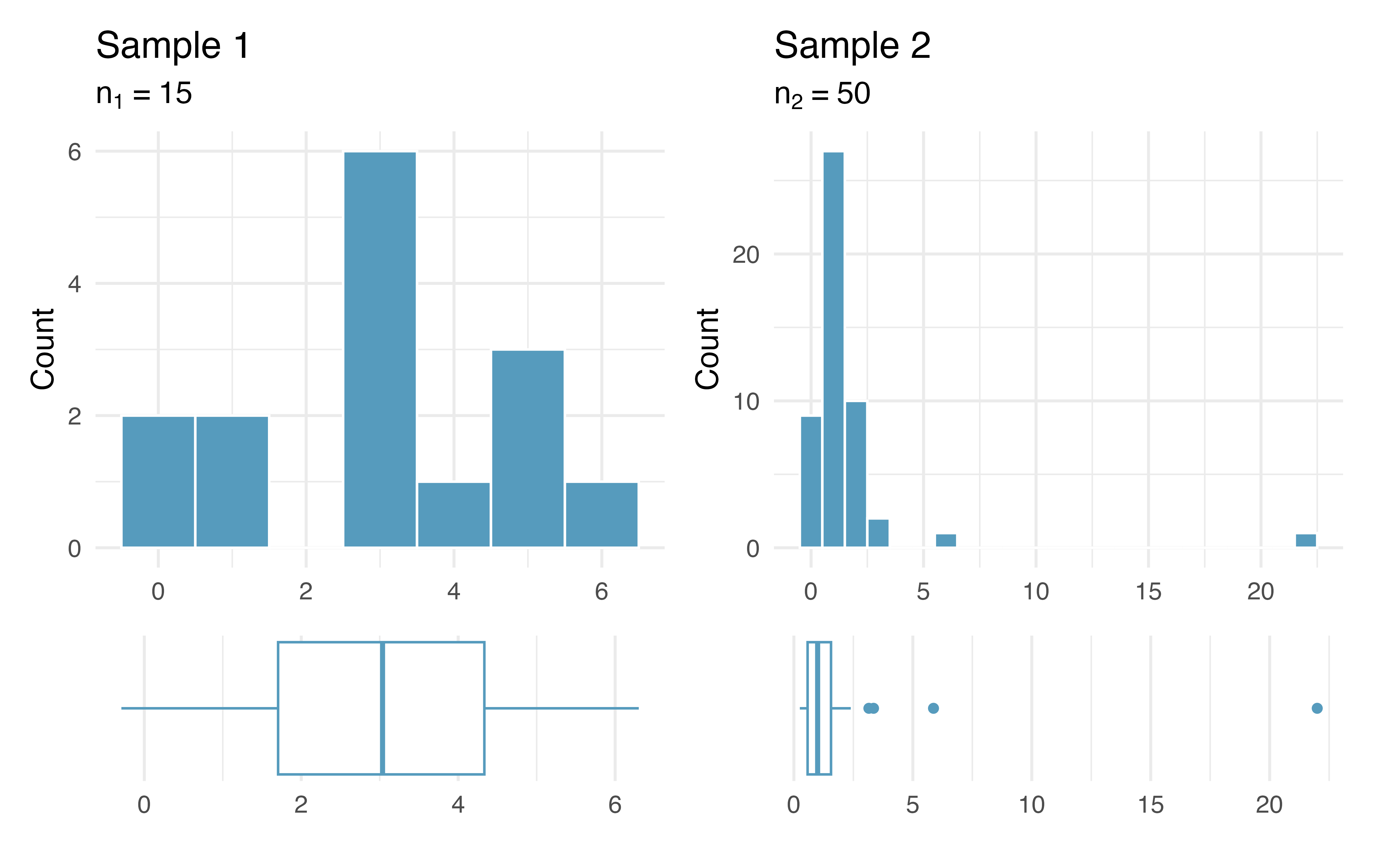
Normality. When a sample is small, we also require that the sample observations come from a normally distributed population. We can relax this condition more and more for larger and larger sample sizes.
– For n < 30, we can plot the data to check to see if the data look normal + there are not clear outliers
– For n > 30, we can’t have obvious (moderate) skew with some outliers
– Good to go for n > 60 unless data are extremely strongly skewed with many outliers
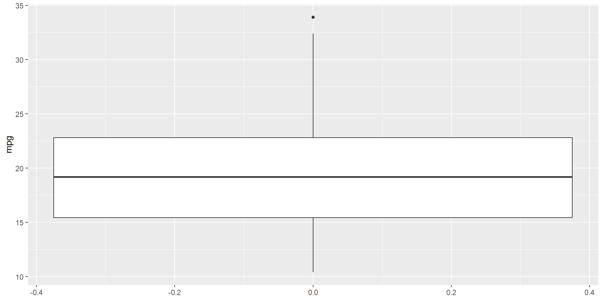
Plot the data
Do we have outliers? What is the shape of these data?
Plot the data
Assumptions
You are not suppose to be an expert your first time. Assessments will be clear cut.
t-distribution
\[ SE = (\frac{\sigma}{\sqrt{n}}) \approx (\frac{s}{\sqrt{n}}) \]
t-distribution
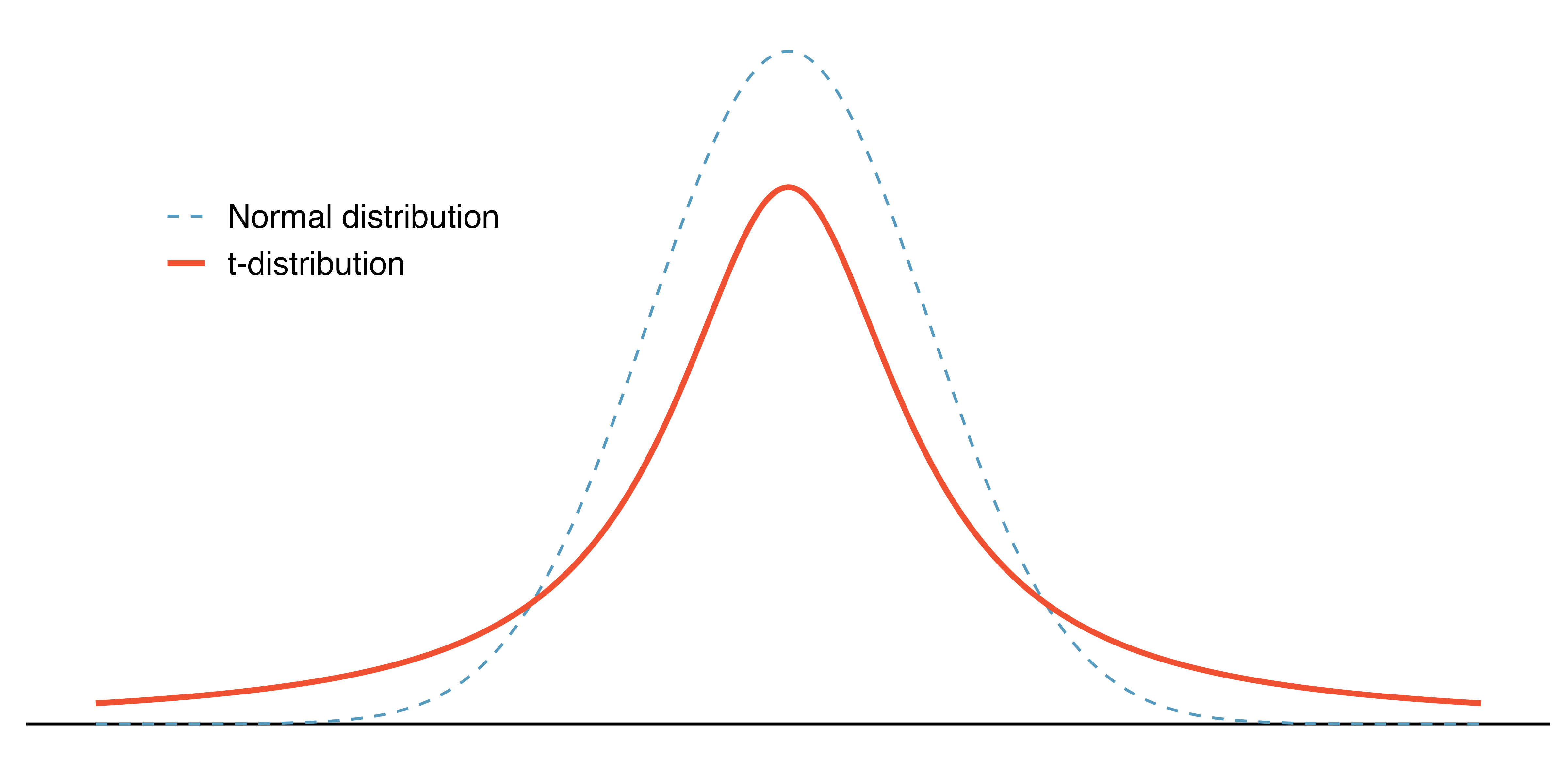
- but we don’t just have one t-distribution
degrees of freedom
The degrees of freedom describes the precise form of the bell-shaped t-distribution
In general, we’ll use a t-distribution with n-1 degrees of freedom to model the sample mean when the sample size is n.
As n increases, our t-distribution approaches a normal distribution!
Show it
standard normal
t-distribution
our t-statistic
Write code to calculate xbar, s, and n
\[ t = \frac{\bar{x} - null}{\frac{s}{\sqrt{n}}} \]
our t-statistic
our t-statistic
\[ t = \frac{20.09 - 12}{\frac{6.03}{\sqrt{32}}} = 7.56 \]
Calculate a p-value
Talk about it
– Decision
– Conclusion
– Interpretation
Simulation
How do we simulate our sampling distribution under the assumption of the null hypothesis?
Let’s go through the steps!
Steps
Find the difference between \(\mu_o\) and \(\bar{x}\)
Subtract this value from each observation
Resample with replacement from your new data
Calculate the sample mean
Repeat this process a large number of times!
Review
Two-sided
Suppose we wanted to conduct a two-sided hypothesis test? What changes?
– How does the research question change?
– How do the hypotheses change?
– How does the statistic change?
– How does the p-value change?
Identify the scenario
I am interested in the difference in flu shots between types of students, and theorize that students living in urban areas get the flu shot more than those in urban areas. Suppose that in a sample of 68 urban students, 42 have had a flu shot and in a sample of 65 rural students, 30 have had a flu shot.
– What are the hypotheses?
– What is our statistic?
Identify the scenario
The price of a popular tennis racket at a national chain store is $179. You wanted to investigate if the same popular tennis racket was cheaper, on average, on Ebay (auction website). Suppose you bought five of the same racket on the Ebay website for the following prices: $163, $138, $201, $155, and $187.
– What are the hypotheses?
– What is our statistic?
