Confidence Inverals
Lecture 10
NC State University
ST 511 - Fall 2024
2024-09-23
Checklist
– Are you keeping up with Slack?
– HW-2 due tonight (11:59pm; 24-hour late window)
– Quiz-5 Wednesday (due Sunday)
Announcements
– As stated on Slack, exercise 1 and 2 are the same office budget context
– Question 5 is an extension question. This is a good example of what you could see on a take-home exam
– This week, we finish up inference with categorical variables. You have (or will have) seen each scenario (hypothesis testing + confidence intervals) using both theory based and simulation based techniques. If we don’t also explicitly cover a scenario, look for a walk through posted
Announcements
Extra credit opportunity: Prepare material for Monday (Sep-30th)
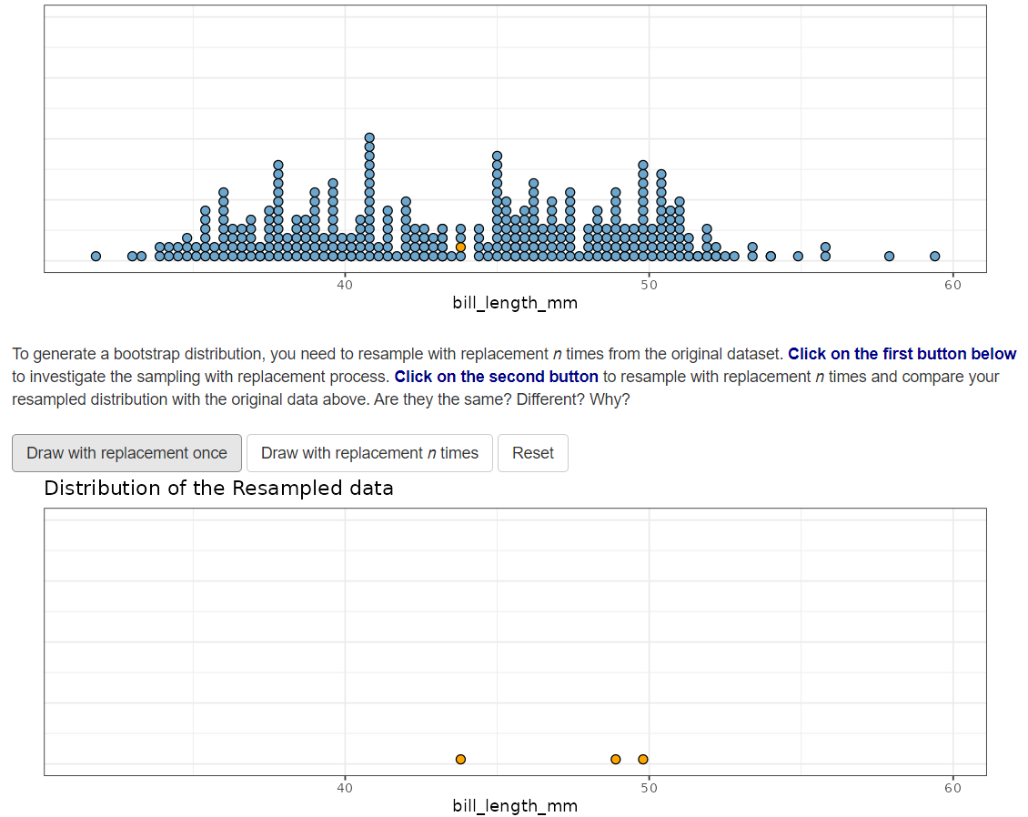
5-10 minute survey Qualtrics survey on if this applet helped!
Warm up question
What do hypothesis tests allow us to accomplish?
Why do researchers conduct hypothesis tests?
Confidence Intervals
Hypothesis testing allowed us to garner evidence if our population parameter is larger, smaller, or different than some value.
We can use confidence intervals to estimate the population parameter we are interested in.
Confidence Intervals: Goal
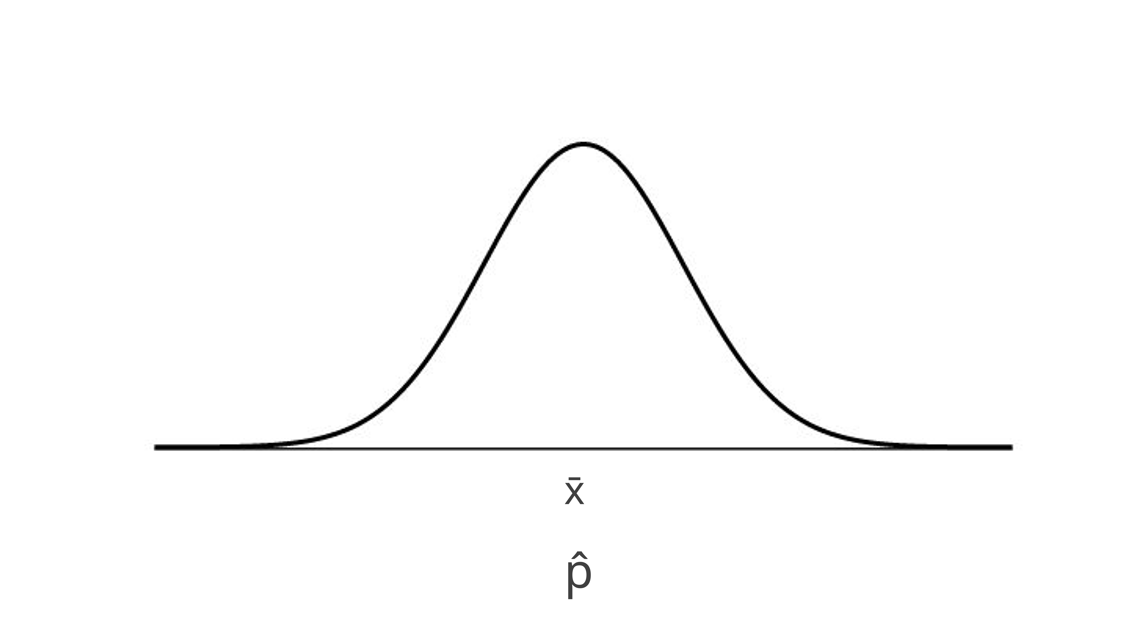
We want to create a sampling distribution around our statistic, and use the standard error (sampling variability) to provide a range of values to estimate our population parameter.
Howling Cow Example
Now instead of conducting a hypothesis test, we want to estimate the number of NC State students that eat ice creme. Recall that our sample statistic was \(\hat{p} = .37\). This is our best guess of \(\pi\), which nobody thinks is actually correct.
Checking assumptions
If our assumptions are valid, then we can estimate the standard error of our statistic.
– Independence (the same as hypothesis testing)
– success-failure condition (sightly different)
success-failure
– Hypothesis testing: successes and failures under the assumption of the null hypothesis
– Confidence interval: successes and failures from our random sample
Howling Cow Assumption Check
– Independence
– Success-failure
\(\hat{p} = .37\)
n = 100
Howling Cow
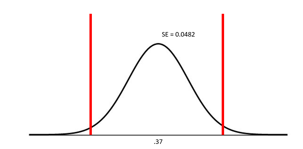
Because our assumptions are satisfied, we can estimate the standard error of our sampling distribution as follows:
\[ SE(\hat{p}) = \sqrt{\frac{\hat{p}*(1-\hat{p})}{n}} \]
\[ SE(\hat{p}) = \sqrt{\frac{.37*.63}{100}} = 0.0482 \]
Creating the confidence interval
Will typically see 90%; 95%; and 99%
Formula: \(\hat{p} \pm\) Margin of Error
Margin of Error = \(z^*\) * SE(\(\hat{p}\))
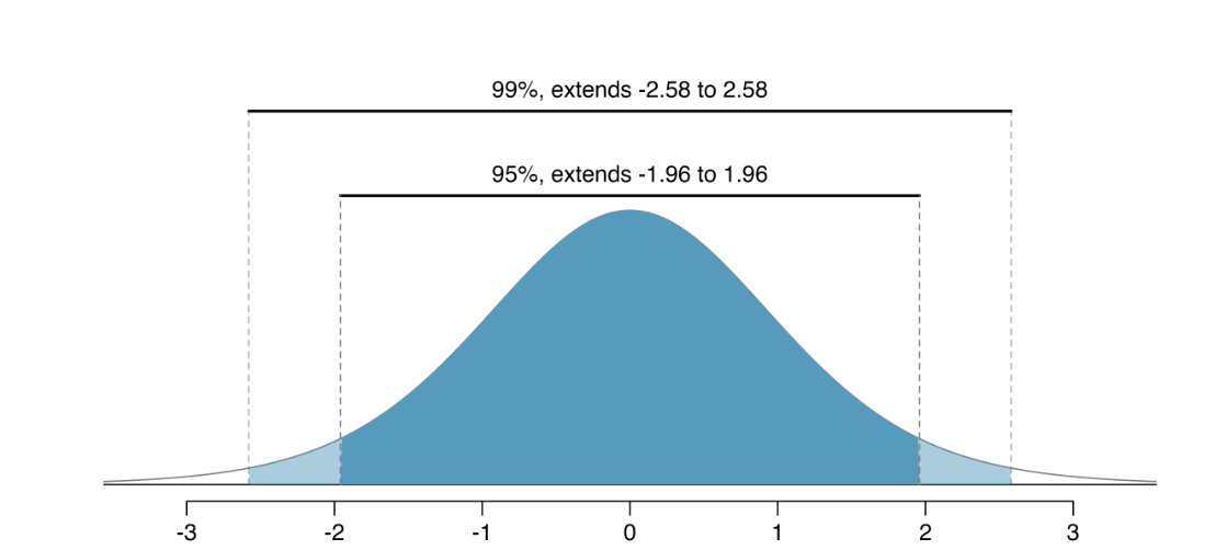
Show, using qnorm, the z* cutoff values for 90%, 95%, and 99%
Calculate a 95% confidence interval
\(\hat{p} \pm z^* * SE(\hat{p})\)
.37 \(\pm\) 1.96*0.0428
.37 \(\pm\) 0.084
.37 + 0.084 = 0.454
.37 - 0.084 = 0.286
(0.286, 0.454)
Talk about it
How do we interpret our confidence interval of (0.286, 0.454)?
We are 95% confident that \(\pi\) is within (0.286, 0.454).
We are 95% confident that the true proportion of NC State students who eat Howling Cow ice creme at dinner is between 0.286 and 0.454.
What about simulation?
Hypothesis testing
\(H_o: \pi = 0.5\)

– Heads = Eat ice creme; Tails = Not eat ice creme
– Flip n times
– Calculate sample proportion
- Do this process a large number of times to estimate the sampling distribution!
Hypothesis testing

– Yellow = Eat ice creme; Blue = not eat ice creme
– Spin n times
– Calculate sample proportion
- Do this process a large number of times to estimate the sampling distribution!
What’s different
We don’t have a null hypothesis….and our goal is to estimate the population parameter
We are going to use bootstrap resample procedures to estimate the sampling distribution
Bootstrap resampling
Resample using our original data
37 yes - Y, Y, Y, Y, Y, ….
63 no - N, N, N, N, N, ….
Let’s demo how the bootstrap resample distribution is created
Steps
Resample with replacement using our original data
n times
Summarize the new resampled data (calculate a statistic)
Do this process a large number of times
sep-23-ae
Results
Would we expect the results of our simulation study to be the same as our theory based method?
Results
We trust them both!
– Theory based (10 success and 10 failures)
– Simulation based (5 success and 5 failures)
New context; same process
Penguins
We are interested in exploring if the species of the penguin is related to the sex of the penguin on the Palmer island. Specifically, we want to know if the species of the penguin impacts the sex of the penguin. We will be looking at the Chinstrap and Gentoo species of penguin.
– What are the variables?
– What is the null and alternative hypothesis?
The Data
The Data
\(\hat{p}_\text{chin}\) = \(\frac{34}{68}\) = .5
\(\hat{p}_\text{gentoo}\) = \(\frac{61}{119}\) = .513
Theory Based Assumptions
Independence (always)
Sample size (success-failure)
What was the assumption for a single variable?
Theory Based Assumptions
\(\hat{p}_\text{pool}\) = \(\frac{\text{total successes}}{\text{total sample size}}\)
\(\hat{p}_\text{pool}\) = \(\frac{\text{34+61}}{\text{187}}\) = 0.508
\[ n1*\hat{p}_\text{pool} > 10 \]
\[ 68*.508 > 10 \]
\[ n1*(1-\hat{p}_\text{pool}) > 10 \]
\[ 68*.492 > 10 \]
Theory Based Assumptions
\[ n2*\hat{p}_\text{pool} > 10 \]
\[ 119*.508 > 10 \]
\[ n2*(1-\hat{p}_\text{pool}) > 10 \]
\[ 119*.492 > 10 \]
- We are good to calculate p-values as we always have before!
